Predicting outbreaks of Dengu Fever using Linear Count Models: Driven Data Competition
by Joe Ganser

Abstract
Dengue fever is a mosquito passed viral infection that is particularly hazardous in tropical environments. Drivendata.co is a website hosting an open source data science competition to find the best model to predict the number of dengue fever cases per day. Using historical infection records in conjunction with environmental data, the competition's goal is to build a count regression model that minimizes the mean absolute error metric. The overall goal of this analysis to break apart the problem and build a basic model. Inspired by Peter Bull's work on the Dengue Fever competition, we build upon this and explore non-linear models. Further research can illicit more accurate models.
I. Problem Statement Goal & Strategy
Predicting the number of daily infections of a disease is a count regression problem with a time series property. This means that the numbers we're predicting can ONLY be positive and finite, and it's possible that some of the variables may evolve over time. To solve this problem, the investigation goes through answering several key questions;
- Is the time series property relevant?
- How does the predictor variables relate to each other and the target variable?
- How would a simple model of predicting the mean/median/zero each day score on our target metric, mean absolute error?
- Are there non-linear relationships between the predictor variable and the target?
- What features are important?
- How do linear models perform?
- How do NON-linear models perform?
Answering these questions will guide use to building a relevant model. The general strategy is to test several models, find the one with the best MAE (mean absolute error) score, and use it to predict on our test set. To experiment with different models, we split the data into train and validation sets.
II. ETL: Extract transform and load the data
The dataset consists of a training dataset and a testing one, which will later be used for forecasting with the best performing model. These are downloaded from AWS S3 buckets and are small enough to be saved locally.
import pandas as pd
import warnings
warnings.filterwarnings('ignore')
test_data_features = 'https://drivendata-prod.s3.amazonaws.com/data/44/public/dengue_features_test.csv?X-Amz-Algorithm=AWS4-HMAC-SHA256&X-Amz-Credential=AKIARVBOBDCYQTZTLQOS%2F20220729%2Fus-east-1%2Fs3%2Faws4_request&X-Amz-Date=20220729T181653Z&X-Amz-Expires=86400&X-Amz-SignedHeaders=host&X-Amz-Signature=c2cabb56ebd41bae9aa5ed99d2ad1b04c587029a3da26b150fedf274b2ec661e'
training_data_features = 'https://drivendata-prod.s3.amazonaws.com/data/44/public/dengue_features_train.csv?X-Amz-Algorithm=AWS4-HMAC-SHA256&X-Amz-Credential=AKIARVBOBDCYQTZTLQOS%2F20220729%2Fus-east-1%2Fs3%2Faws4_request&X-Amz-Date=20220729T181653Z&X-Amz-Expires=86400&X-Amz-SignedHeaders=host&X-Amz-Signature=86638e7bbf2f4d0e35e91314a47ae3d94270b000a7255fa48a6eac87ffb3ecfb'
training_data_labels = 'https://drivendata-prod.s3.amazonaws.com/data/44/public/dengue_labels_train.csv?X-Amz-Algorithm=AWS4-HMAC-SHA256&X-Amz-Credential=AKIARVBOBDCYQTZTLQOS%2F20220729%2Fus-east-1%2Fs3%2Faws4_request&X-Amz-Date=20220729T181653Z&X-Amz-Expires=86400&X-Amz-SignedHeaders=host&X-Amz-Signature=01891140cdf2983b4155e439da14527ccb65d4a311009564bec5e0b01d23cf9c'
try:
    df_test = pd.read_csv(test_data_features)
    df_train_features = pd.read_csv(training_data_features)
    df_train_labels = pd.read_csv(training_data_labels)
    df_train = df_train_features.merge(df_train_labels,on=['city','year','weekofyear'])
except:
    df_train = pd.read_csv('train.csv',index_col=0)
    df_test = pd.read_csv('test.csv',index_col=0)
target = 'total_cases'
df_train.head()
| city | year | weekofyear | week_start_date | ndvi_ne | ndvi_nw | ndvi_se | ndvi_sw | precipitation_amt_mm | reanalysis_air_temp_k | ... | reanalysis_relative_humidity_percent | reanalysis_sat_precip_amt_mm | reanalysis_specific_humidity_g_per_kg | reanalysis_tdtr_k | station_avg_temp_c | station_diur_temp_rng_c | station_max_temp_c | station_min_temp_c | station_precip_mm | total_cases |
|---|---|---|---|---|---|---|---|---|---|---|---|---|---|---|---|---|---|---|---|---|
| 0 | sj | 1990 | 18 | 1990-04-30 | 0.122600 | 0.103725 | 0.198483 | 0.177617 | 12.42 | 297.572857 | ... | 73.365714 | 12.42 | 14.012857 | 2.628571 | 25.442857 | 6.900000 | 29.4 | 20.0 | 16.0 |
| 1 | sj | 1990 | 19 | 1990-05-07 | 0.169900 | 0.142175 | 0.162357 | 0.155486 | 22.82 | 298.211429 | ... | 77.368571 | 22.82 | 15.372857 | 2.371429 | 26.714286 | 6.371429 | 31.7 | 22.2 | 8.6 |
| 2 | sj | 1990 | 20 | 1990-05-14 | 0.032250 | 0.172967 | 0.157200 | 0.170843 | 34.54 | 298.781429 | ... | 82.052857 | 34.54 | 16.848571 | 2.300000 | 26.714286 | 6.485714 | 32.2 | 22.8 | 41.4 |
| 3 | sj | 1990 | 21 | 1990-05-21 | 0.128633 | 0.245067 | 0.227557 | 0.235886 | 15.36 | 298.987143 | ... | 80.337143 | 15.36 | 16.672857 | 2.428571 | 27.471429 | 6.771429 | 33.3 | 23.3 | 4.0 |
| 4 | sj | 1990 | 22 | 1990-05-28 | 0.196200 | 0.262200 | 0.251200 | 0.247340 | 7.52 | 299.518571 | ... | 80.460000 | 7.52 | 17.210000 | 3.014286 | 28.942857 | 9.371429 | 35.0 | 23.9 | 5.8 |
III. Exploratory data analysis (EDA)
It's important that we explore the structure of the data set to build a strategy for solving this problem. Let begin by exploring the time series of total cases, and it's histogram. The goal here is to examine relationships between predictors and the target, as well as determine how the time series evolved.
III.A Examining the target variable; total_cases
Lets evaluate the time series and histogram of our target variable.
import matplotlib.pyplot as plt
def plot_feature_timeseries(data,feature):
    time_series = data[['city','week_start_date',feature]]
    time_series['week_start_date'] = pd.to_datetime(time_series['week_start_date'])
    time_series.set_index('week_start_date',inplace=True)
    plt.figure(figsize=(18,8))
    plt.title('both cities',fontsize=20)
    plt.plot(time_series[time_series['city']=='sj'][feature],label='SJ',color='blue')
    plt.plot(time_series[time_series['city']=='iq'][feature],label='IQ',color='red')
    plt.legend(fontsize=20)
    plt.ylabel(feature,fontsize=20)
    plt.xticks(fontsize=20)
    plt.show()

plot_feature_timeseries(df_train,'total_cases')
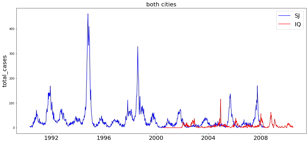
We can see from the start that this is a cyclic time series count regression problem. It's possible that seasonal trends are at play, and it's important to determine if there is an evolution in values over time (stationarity).
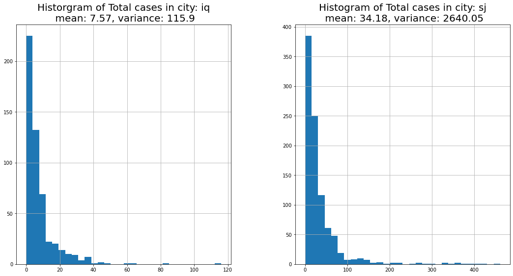
Our target variable is total_cases, and in any regression problem it's always good to evaluate the histogram of our target.
plt.figure(figsize=(18,9))
plt.subplot(1,2,1)
iq_mean = round(df_train[df_train['city']=='iq']['total_cases'].mean(),2)
iq_var = round(df_train[df_train['city']=='iq']['total_cases'].var(),2)
plt.title('Historgram of Total cases in city: iq\n mean: {}, variance: {}'.format(iq_mean,iq_var),fontsize=20)
df_train[df_train['city']=='iq']['total_cases'].hist(bins=30)
plt.subplot(1,2,2)
sj_mean = round(df_train[df_train['city']=='sj']['total_cases'].mean(),2)
sj_var = round(df_train[df_train['city']=='sj']['total_cases'].var(),2)
plt.title('Histogram of Total cases in city: sj\n mean: {}, variance: {}'.format(sj_mean,sj_var),fontsize=20)
df_train[df_train['city']=='sj']['total_cases'].hist(bins=30)
plt.subplots_adjust(wspace=0.3)
plt.show()
III.B Data cleaning
The data has some missing values, and due to the nature of being a time series across different cities, the correct approach to fill these data points would be to use the foward fill method.
iq = df_train[df_train['city']=='iq']
sj = df_train[df_train['city']=='sj']
sj.fillna(method='ffill', inplace=True)
iq.fillna(method='ffill', inplace=True)
df_train = pd.concat([sj,iq],axis=0)
df_train.head()
5 rows × 25 columns
| city | year | weekofyear | week_start_date | ndvi_ne | ndvi_nw | ndvi_se | ndvi_sw | precipitation_amt_mm | reanalysis_air_temp_k | ... | reanalysis_relative_humidity_percent | reanalysis_sat_precip_amt_mm | reanalysis_specific_humidity_g_per_kg | reanalysis_tdtr_k | station_avg_temp_c | station_diur_temp_rng_c | station_max_temp_c | station_min_temp_c | station_precip_mm | total_cases |
|---|---|---|---|---|---|---|---|---|---|---|---|---|---|---|---|---|---|---|---|---|
| 0 | sj | 1990 | 18 | 1990-04-30 | 0.122600 | 0.103725 | 0.198483 | 0.177617 | 12.42 | 297.572857 | ... | 73.365714 | 12.42 | 14.012857 | 2.628571 | 25.442857 | 6.900000 | 29.4 | 20.0 | 16.0 |
| 1 | sj | 1990 | 19 | 1990-05-07 | 0.169900 | 0.142175 | 0.162357 | 0.155486 | 22.82 | 298.211429 | ... | 77.368571 | 22.82 | 15.372857 | 2.371429 | 26.714286 | 6.371429 | 31.7 | 22.2 | 8.6 |
| 2 | sj | 1990 | 20 | 1990-05-14 | 0.032250 | 0.172967 | 0.157200 | 0.170843 | 34.54 | 298.781429 | ... | 82.052857 | 34.54 | 16.848571 | 2.300000 | 26.714286 | 6.485714 | 32.2 | 22.8 | 41.4 |
| 3 | sj | 1990 | 21 | 1990-05-21 | 0.128633 | 0.245067 | 0.227557 | 0.235886 | 15.36 | 298.987143 | ... | 80.337143 | 15.36 | 16.672857 | 2.428571 | 27.471429 | 6.771429 | 33.3 | 23.3 | 4.0 |
| 4 | sj | 1990 | 22 | 1990-05-28 | 0.196200 | 0.262200 | 0.251200 | 0.247340 | 7.52 | 299.518571 | ... | 80.460000 | 7.52 | 17.210000 | 3.014286 | 28.942857 | 9.371429 | 35.0 | 23.9 | 5.8 |
III.C Time series and stationarity
This appears to be a time series count-regression problem. In any time series it's important to determine if there is an existing trend in the time series - i.e. if it's stationary. Stationarity in time series indicates if the average is constant in time. To determine stationarity, we can use the augmented dickey fuller test. Thus we perform the augmented dickey fuller test on the time series for both cities.
If it's determined that all columns are stationary, we can treat this as a typical count-regression problem.
from statsmodels.tsa.stattools import adfuller
def dickey_fuller_test(data):
    test_statistic,p_value,lags_used,observations,critical_values,icbest = adfuller(data)
    metric = 'test statistic: {}, p_value: {}'.format(test_statistic,p_value)
    for key in sorted(critical_values.keys()):
        alpha = float(key.replace('%',''))/100
        critical = float(critical_values[key])
        if test_statistic<=critical and p_value<=alpha:
            metric2 = '{}:{}'.format(key,critical_values[key])
            return 'Stationary Series, Reject Null Hypothesis;\n '+metric+'\n '+metric2
    return 'Fail to reject null hypothesis, stationary series: '+metric
The data comes in different contexts: one time series for each city in the data studied. Hence we should run all the evaluations in the following contexts;
- City IQ
- City SJ
- Both cities, combined
Now lets determine if the target, total_cases, is stationary.
time_series = df_train[['city','week_start_date','total_cases']]
time_series['week_start_date'] = pd.to_datetime(time_series['week_start_date'])
for city in ['sj','iq','both']:
    print('City: {}'.format(city))
    if city=='both':
        print(dickey_fuller_test(time_series['total_cases']))
    else:
        print(dickey_fuller_test(time_series[time_series['city']==city]['total_cases']))
    print('\n')
City: sj
Stationary Series, Reject Null Hypothesis;
 test statistic: -6.650077901931189, p_value: 5.1473186737592894e-09
 1%:-3.4374315551464734


City: iq
Stationary Series, Reject Null Hypothesis;
 test statistic: -6.085428681900057, p_value: 1.0672522948401663e-07
 1%:-3.4431115411022146


City: both
Stationary Series, Reject Null Hypothesis;
 test statistic: -6.6232582356851655, p_value: 5.963285375798725e-09
 1%:-3.434889827343955
Now we should run the test for stationarity across all the other features, in each city context.
features = [j for j in df_train.columns if j not in ['total_cases','week_start_date','city','year','weekofyear']]
for col in features:
    _ = df_train[['city','week_start_date',col]]
    _['week_start_date'] = pd.to_datetime(_['week_start_date'])
    for city in ['sj','iq','both']:
        if city=='both':
            test = dickey_fuller_test(_[col])
        else:
            test = dickey_fuller_test(_[_['city']==city][col])
        if 'Fail' in test:
            print('Feature: {} in cities: {} is non-stationary'.format(col,city))
Feature: station_diur_temp_rng_c in cities: both is non-stationary
We see the the only feature regarded as non-stationary is station_diur_temp_rng_c. Lets graphically see what may cause this.
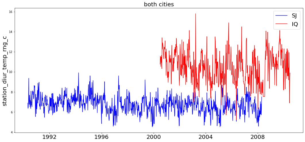
Clearly, this isn't do to a trend evolving over time, but only due to the feature's average value being different for each city. In our series of tests, we also evaluated the time series being stationary when evaluating on each city individually. Thus for all intensive purposes, we can regard this feature as infract stationary.
III.D Correlations between features and target
Even though this is not a gaussian based regression problem, where the errors are assumed to be normally distributed, we can still inquite on the pearson correlation between each feature and our target variable total_cases. A bar plot showing the correlation of each feature with the target, in the context of each city can help us.
import numpy as np
import seaborn as sns
sj_corrs = {}
iq_corrs = {}
for col in df_train.columns:
    if col not in ['year','week_start_date','city','total_cases']:
        _ = df_train[df_train['city']=='sj'][[col,'total_cases']]
        sj = np.corrcoef(_[col],_['total_cases'])[0][1]
        sj_corrs[col]=[sj]
        __ = df_train[df_train['city']=='iq'][[col,'total_cases']]
        iq = np.corrcoef(__[col],__['total_cases'])[0][1]
        iq_corrs[col]=[iq]
plt.figure(figsize=(12,12))
plt.title('Pearson correlations for each feature with total_cases',fontsize=20)
sns.barplot(x=0, y='index', data=pd.DataFrame(sj_corrs).transpose().reset_index(), color="b",label='sj')
sns.barplot(x=0, y='index', data=pd.DataFrame(iq_corrs).transpose().reset_index(), color="r",label='iq')
plt.legend(fontsize=20)
plt.show()
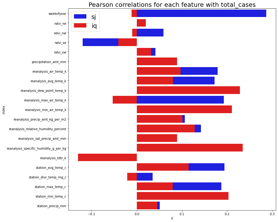
From this plot we can see that most features are weakly correlated with the target. Some features have different correlations for different cities. For example, weekofyear has almost no correlation in city iq, but very strong correlation with sj. Perhaps this is due to geographical positioning of the cities, and seasonal effects may be more extreme in some locations over others.
III.E Correlations between features (heat map)
iq_features = df_train[df_train['city']=='iq'].drop(['week_start_date','year'],axis=1).corr()
sj_features = df_train[df_train['city']=='sj'].drop(['week_start_date','year'],axis=1).corr()
plt.figure(figsize=(10,20))
plt.subplot(2,1,1)
plt.title('Heat map for features in city IQ',fontsize=20)
sns.heatmap(iq_features)
plt.subplot(2,1,2)
plt.title('Heat map for features in city SJ',fontsize=20)
sns.heatmap(sj_features)
plt.subplots_adjust(hspace=0.7)
plt.show()
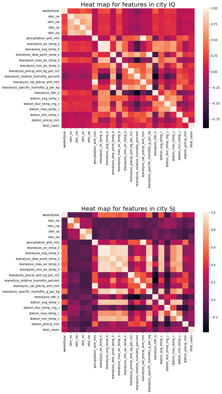
A few examples;
Correlations between different features range widely, between 0.997 (max) and -0.896 (min). Thus this may indicate colinearity between features that could be problematic for linear models.
For city SJ;
* weekofyear has negative correlation with reanalysis_air_temp_k of 0.904
* reanalysis_dew_point_temp_k has negative correlation with reanalysis_tdtr_k of -0.374
For city IQ
* weekofyear has negative correlation with reanalysis_specific_humidity_g_per_kg of 0.997
* reanalysis_dew_point_temp_k has positive correlation with reanalysis_tdtr_kc of -0.896
III.F Establishing a baseline: performance of a constant model
In a regression problem, one strategy to establish a baseline model is to ask the following questions;
- How accurate would our model be if we only predicted the mean?
- Or if we only predicted median?
- Or if we only predicted zero?
What would the loss and performance metrics be for this? Using these metrics, we can conclude any model that performance worse than this is by definition no better than simply guessing the mean/median/zero for every row.
We should answer these questions in the context of each city, and the cities combined.
from sklearn.metrics import mean_absolute_error
def scores_of_bad_models(df):
    predict_median = [np.median(df['total_cases']) for i in range(len(df))]
    predict_mean = [df['total_cases'].mean() for i in range(len(df))]
    predict_zero = [0 for i in range(len(df))]
    predict_mean_error = round(mean_absolute_error(df['total_cases'],predict_mean),2)
    predict_zero_error = round(mean_absolute_error(df['total_cases'],predict_zero),2)
    predict_median_error = round(mean_absolute_error(df['total_cases'],predict_median),2)
    return predict_mean_error,predict_zero_error,predict_median_error

datasets = [df_train,df_train[df_train['city']=='sj'],df_train[df_train['city']=='iq']]
scores = {}
for i in range(3):
    if i==0:
        name = 'both'
    elif i==1:
        name = 'sj'
    elif i==2:
        name = 'iq'
    scores[name] = [*scores_of_bad_models(datasets[i])]

scores = pd.DataFrame(scores).transpose()
scores.columns = ['predict_mean','predict_zero','predict_median']
scores['min'] = scores.apply(lambda x: x.min(),axis=1)
scores.index.name='cities'
scores
| cities | predict_zero | predict_median | min |
|---|---|---|---|
| both | 23.00 | 24.68 | 19.88 |
| sj | 28.35 | 34.18 | 24.71 |
| iq | 6.68 | 7.57 | 6.05 |
Thus for both cities combined, the predicting the median every day would yield a mean_absolute_error of 19.88. For city SJ it's 24.71 and IQ it's 6.05. Thus any useful model should have a mean absolute error lower than these values.
III.G Selecting the right linear model
This is a count regression problem, which means that at no time should we expect our model or measurements to be less than zero. Some other examples of similar problems are;
- Number of hurricanes per year
- Number of traffic accidents per month
- Customer visits to a website per day
Hence to measure -5 negative cases of dengu fever on a given day really has no meaning. There are two linear model approaches to solving problems like this, each with different assumptions.
- Poisson Regression
- Negative binomial distribution
Poisson regression assumes that the average count per day will equal the variance. If this assumption is invalidated by our data, negative binomial distribution will be the appropriate model to use.
From the section above "examining the target variable", we know that;
-
City IQ:
- mean: 7.57 cases/day
- variance: 115.9
-
City SJ:
- mean: 34.18 cases/day
- variance: 2640
Hence the variance far exceeds the mean, so Negative binomial distribution is most relevant. This is known as over dispersion.
III.G1 Linear modeling: Predictability of each feature versus the target
One technique in feature selection is to examine the predictability using each feature versus the target variable, using a linear model (negative binomial distribution, hyper parameters tuned). This gives us an estimate of the usefulness of each feature in predicting the target, and we can eliminate features with poor predictability. This technique is limited to cases where the relationships between variabels are linear, but does give some useful insight. This script is inspired by source [1].
from statsmodels.tools import eval_measures
import statsmodels.formula.api as smf
import statsmodels.api as sm
def negative_binomial_one_feature(train,test,city,param_grid,feature):
    model_formula = "total_cases ~ {}".format(feature)
    best_alpha = 0
    best_score = 1000
    for alpha in param_grid:
        model = smf.glm(formula=model_formula,data=train,family=sm.families.NegativeBinomial(alpha=alpha))
        results = model.fit()
        predictions = results.predict(test).astype(int)
        score = eval_measures.meanabs(predictions, test.total_cases)
        if score < best_score:
            best_alpha = alpha
            best_score = score
    metrics = {'city':city,'best_MAE':best_score,'alpha':best_alpha,'feature':feature}
    return metrics


def feature_tests(data,features,param_grid):
    mask = np.random.rand(len(data))<0.8
    train = data[mask]
    test = data[~mask]
    results = []
    cities = ['sj','iq']
    for feature in features:
        for element in range(3):
            tr,te = train.copy(),test.copy()
            if element in [0,1]:
                city = cities[element]
                tr = tr[tr['city']==city]
                te = te[te['city']==city]
            else:
                city = 'both'
            tr.drop('city',axis=1,inplace=True)
            te.drop('city',axis=1,inplace=True)
            result = negative_binomial_one_feature(tr,te,city,param_grid,feature)
            results.append(result)
    return pd.DataFrame(results)

features = [j for j in df_train.columns if j not in ['city','year','week_start_date',target]]
param_grid = np.arange(0.001,20,0.05)
feature_results = feature_tests(df_train,features,param_grid)
feature_results.head()
| feature | city | best_MAE | alpha |
|---|---|---|---|
| weekofyear | sj | 23.384181 | 5.701 |
| weekofyear | iq | 6.741935 | 0.001 |
| weekofyear | both | 19.374074 | 1.601 |
| ndvi_ne | sj | 25.005650 | 0.001 |
| ndvi_ne | iq | 6.741935 | 0.001 |
Now we have a comparison of each the mean absolute error of each feature versus the target, where the linear model is fitted with an optimal hyper-parameter. From this we can look at the histogram of scores, and see how many features had a mean absolute error less than that of a constant model. Features that performed better than a constant model are probably useful, ones that didn't may not be.
plt.figure(figsize=(18,6))
plt.subplot(1,3,1)
plt.title('Feature scores for city: sj \n min MAE for constant model: {}'.format(scores.loc['sj']['min']))
feature_results[feature_results['city']=='sj']['best_MAE'].hist(bins=len(features))
plt.axvline(scores.loc['sj']['min'],label='median prediction error',color='red')
plt.xlabel('MAE',fontsize=20)
plt.ylabel('count',fontsize=20)
plt.legend()
plt.subplot(1,3,2)
plt.title('Feature scores for city: iq \n min MAE for constant model: {}'.format(scores.loc['iq']['min']))
feature_results[feature_results['city']=='iq']['best_MAE'].hist(bins=len(features))
plt.axvline(scores.loc['iq']['min'],label='median prediction error',color='red')
plt.subplot(1,3,3)
plt.title('Feature scores for both cities combined \n min MAE for constant model: {}'.format(scores.loc['both']['min']))
feature_results[feature_results['city']=='both']['best_MAE'].hist(bins=len(features))
plt.axvline(scores.loc['both']['min'],label='median prediction error',color='red')
plt.show()
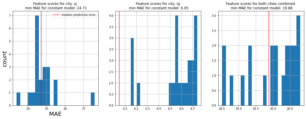
From the graphs above we can see that a negative binomial distribution on each feature versus the target usually doesn't perform any better than simply guessing mean/median/zero every day.
Thus we can hypothesize; linear models probably have poor predictability on this data set.
III.G2 Feature selection
For there are some features that had a MAE better than the minimum MAE provided by a constant model. Another hypothesis can be formed suggesting that these features may be useful and a linear model with them only may provide some good performance. Lets see what these features are.
min_scores = pd.DataFrame(scores['min']).reset_index()
feature_results_joined = feature_results.merge(min_scores,left_on='city',right_on='cities')[['best_MAE','cities','alpha','min','feature']]
key_features = feature_results_joined[feature_results_joined['best_MAE']<=feature_results_joined['min']]
key_features_list = list(set(key_features['feature']))
key_features
| best_MAE | cities | alpha | min | feature |
|---|---|---|---|---|
| 23.384181 | sj | 5.701 | 24.71 | weekofyear |
| 24.502825 | sj | 0.151 | 24.71 | precipitation_amt_mm |
| 24.531073 | sj | 0.001 | 24.71 | reanalysis_air_temp_k |
| 24.587571 | sj | 0.001 | 24.71 | reanalysis_avg_temp_k |
| 24.186441 | sj | 0.201 | 24.71 | reanalysis_dew_point_temp_k |
| 24.406780 | sj | 0.801 | 24.71 | reanalysis_max_air_temp_k |
| 24.451977 | sj | 0.001 | 24.71 | reanalysis_relative_humidity_percent |
| 24.502825 | sj | 0.151 | 24.71 | reanalysis_sat_precip_amt_mm |
| 24.141243 | sj | 0.001 | 24.71 | reanalysis_specific_humidity_g_per_kg |
| 24.525424 | sj | 0.001 | 24.71 | station_min_temp_c |
| 24.581921 | sj | 0.901 | 24.71 | station_precip_mm |
| 19.374074 | both | 1.601 | 19.88 | weekofyear |
| 18.822222 | both | 0.001 | 19.88 | reanalysis_air_temp_k |
| 19.803704 | both | 0.051 | 19.88 | reanalysis_avg_temp_k |
| 18.511111 | both | 9.701 | 19.88 | reanalysis_min_air_temp_k |
| 18.522222 | both | 1.101 | 19.88 | reanalysis_tdtr_k |
| 19.359259 | both | 0.001 | 19.88 | station_diur_temp_rng_c |
| 19.085185 | both | 1.151 | 19.88 | station_min_temp_c |
The data frame above provides the results where the negative binomial distribution on the feature versus total_cases performed better than guessing the median. These feature were;
['reanalysis_max_air_temp_k',
 'reanalysis_min_air_temp_k',
 'reanalysis_avg_temp_k',
 'reanalysis_air_temp_k',
 'reanalysis_specific_humidity_g_per_kg',
 'station_diur_temp_rng_c',
 'reanalysis_dew_point_temp_k',
 'station_min_temp_c',
 'reanalysis_tdtr_k',
 'weekofyear',
 'station_precip_mm',
 'precipitation_amt_mm',
 'reanalysis_relative_humidity_percent',
 'reanalysis_sat_precip_amt_mm']
IV Modelling
The strategy for modeling is to begin with simple linear models, evaluate their performance and then attempt non-linear ones such as random forest regression.
IV.A Modelling: Negative Binomial distribution
We previously established a baseline performance of what guessing the median value every day would be, and we also identified. Now lets run experiments using negative binomial distribution on;
- top features from the last step
- all the features
def negative_binomial_models(data,param_grid,*train_features,return_predictions=False):
    if 'city' in data.columns:
        data['city']=data['city'].apply(lambda x: 1 if x=='sj' else 0)
    mask = np.random.rand(len(data))<0.8
    train = data[mask]
    test = data[~mask]

    model_formula = "total_cases ~"
    for index,f in enumerate([j for j in train_features if j!='total_cases']):
        if index==0:
            model_formula = model_formula+" {}".format(f)
        else:
            model_formula = model_formula+" + {}".format(f)
    best_alpha = None
    best_score = 1000

    for alpha in param_grid:
        model = smf.glm(formula=model_formula,data=train,family=sm.families.NegativeBinomial(alpha=alpha))
        results = model.fit()
        predictions = results.predict(test).astype(int)
        score = eval_measures.meanabs(predictions, test.total_cases)
        if score < best_score:
            best_alpha = alpha
            best_score = score
    # Step 3: refit on entire dataset
    best_model = smf.glm(formula=model_formula,data=train,family=sm.families.NegativeBinomial(alpha=best_alpha))
    best_results = best_model.fit()
    predictions_train = best_results.predict(train).astype(int)
    predictions_test = best_results.predict(test).astype(int)
    score_train = eval_measures.meanabs(predictions_train, train.total_cases)
    score_test = eval_measures.meanabs(predictions_test, test.total_cases)
    metrics = {'MAE_test':score_train,'MAE_train':score_test,'alpha':best_alpha}
    return metrics
Tune and test negative binomial distribution on the key features observed before.
{'MAE_test': 19.004198152812762,
 'MAE_train': 18.724528301886792,
 'alpha': 0.051000000000000004}
Tune and test negative binomial distribution on all the features.
all_features = [j for j in df_train.columns if j not in ['year','week_start_date',target]]
negative_binomial_models(df_train,param_grid,*all_features)
{'MAE_test': 17.706837606837606,
 'MAE_train': 21.377622377622377,
 'alpha': 0.101}
From these results we can see that although the model's performance on both a train and test set indicates a reasonably good fit, but the MAE performs approximately the same as guessing the median. Thus its worth investigating a better performing model than negative binomial distribution.
IV.B Modelling: Random Forest Regression
Random forest regression is a good model for data sets that contain non-linearities between features. As a first experiment. It's also good to use a standard scalarizer of our data before putting it into the random forest model.
from sklearn.ensemble import RandomForestRegressor
from sklearn.metrics import mean_absolute_error
from sklearn.pipeline import Pipeline
from sklearn.preprocessing import StandardScaler
from sklearn.model_selection import train_test_split
import random

def preprocess_data(data):
    for c in ['week_start_date','year']:
        if c in data.columns:
            data.drop(c,axis=1,inplace=True)
    data['city']=data['city'].apply(lambda x: 1 if x=='sj' else 0)
    if target in data.columns:
        X = data.drop(target,axis=1)
        y = data[target]
    else:
        X = data
        y = None
    return X,y


def split_and_preprocess_data(data):
    X,y = preprocess_data(data)
    X_train, X_val, y_train, y_test = train_test_split(X, y, test_size=0.2, random_state=43)
    return X_train, X_val, y_train, y_val

criterion = ["poisson","mse","mae"]
max_depth = [None,20,25,30,35]
max_features = ["sqrt", "log2", None]
num_estimators = [10,50,100,150]

best_err = 1000
best_params = []

X_train, X_val, y_train, y_val = split_and_preprocess_data(df_train.copy())
for c in criterion:
    for d in max_depth:
        for f in max_features:
            for n in num_estimators:
                rf = RandomForestRegressor(n_estimators=n,criterion=c,max_depth=d,max_features=f)
                pipe_rf = Pipeline([('scaler', StandardScaler()), ('rf',rf)])
                pipe_rf.fit(X_train,y_train)
                y_pred = pipe_rf.predict(X_test)
                y_pred[y_pred==np.inf]=0
                y_pred[y_pred<0]=0
                err = mean_absolute_error(y_test,y_pred)
                if err<best_err:
                    best_err = err
                    if len(best_params)!=0:
                        best_params.pop()
                    best_params.append([c,d,f,n])

print(best_err)
print(best_params)
16.54417808219178
[['mse', 35, None, 10]]
IV.B1 Random Forest: Feature selection
Our MAE (for this split) is 16.54. This is reasonably good and better than the negative binomial distribution. Using these hyperparameters, lets fit the model to take advance of random forest's feature selection.
c='mse'
d=30
f=None
n=50
rf = RandomForestRegressor(n_estimators=n,criterion=c,max_depth=d,max_features=f)
pipe_rf = Pipeline([('scaler', StandardScaler()), ('rf',rf)])
pipe_rf.fit(X_train,y_train)

for feature in zip(X_train.columns, rf.feature_importances_):
    print(feature)
('city', 0.00012123375843353865)
('weekofyear', 0.0884120168882518)
('ndvi_ne', 0.018704338094528178)
('ndvi_nw', 0.02330064085826595)
('ndvi_se', 0.3065804669674904)
('ndvi_sw', 0.08197494560635799)
('precipitation_amt_mm', 0.008394869826651807)
('reanalysis_air_temp_k', 0.01718239611866463)
('reanalysis_avg_temp_k', 0.019715048212381053)
('reanalysis_dew_point_temp_k', 0.04598412742970319)
('reanalysis_max_air_temp_k', 0.023837285355508442)
('reanalysis_min_air_temp_k', 0.10103776364819778)
('reanalysis_precip_amt_kg_per_m2', 0.032496353106185906)
('reanalysis_relative_humidity_percent', 0.015229479597685027)
('reanalysis_sat_precip_amt_mm', 0.005335078003527012)
('reanalysis_specific_humidity_g_per_kg', 0.035410600175340604)
('reanalysis_tdtr_k', 0.04086107229416256)
('station_avg_temp_c', 0.02208406820316571)
('station_diur_temp_rng_c', 0.016308194900887744)
('station_max_temp_c', 0.04946073934079644)
('station_min_temp_c', 0.014044667116736333)
('station_precip_mm', 0.033524614497077845)
X_train, X_val, y_train, y_val = split_and_preprocess_data(df_train.copy())
rf = RandomForestRegressor(n_estimators=50,criterion='mse',max_depth=None,max_features=None)
pipe = Pipeline([('scaler', StandardScaler()), ('rf',rf)])
pipe.fit(X_train,y_train)


y_pred_val = pipe.predict(X_val)
y_pred_train = pipe.predict(X_train)
y_pred_val[y_pred_val == np.inf] = 0
y_pred_val[y_pred_val<0]=0
y_pred_train[y_pred_train == np.inf] = 0
y_pred_train[y_pred_train<0]=0
err_val = mean_absolute_error(y_val,y_pred_val)
err_train = mean_absolute_error(y_train,y_pred_train)
print(err_val)
print(err_train)
17.56821917808219
5.864226804123711
IV.B2 Random forest results * MAE validation set: 17.56 * MAE train set: 5.86
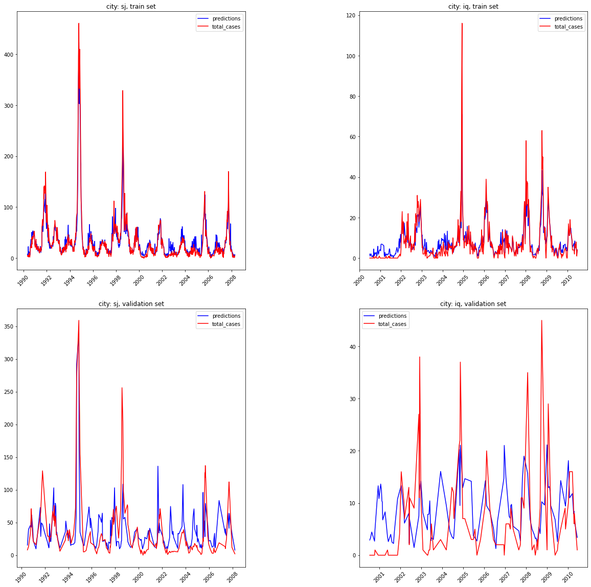
Despite the model being overfit, lets plot this and see how the predictions compare for the train and validation sets.
val = pd.concat([X_val,y_val],axis=1)
train = pd.concat([X_train,y_train],axis=1)
val['predictions'] = y_pred_val
train['predictions'] = y_pred_train
indices = df_train[['week_start_date','total_cases','weekofyear','year','city']]
val_result = val.join(indices,on=None,lsuffix='Left')[['total_cases','predictions','week_start_date','city']]#.set_index('week_start_date')
val_result.sort_values(by='week_start_date',inplace=True)
val_result['data_set'] = 'validation'
train_result = train.join(indices,on=None,lsuffix='Left')[['total_cases','predictions','week_start_date','city']]
train_result.sort_values(by='week_start_date',inplace=True)
train_result['data_set'] = 'train'
predictions = pd.concat([val_result,train_result],axis=0)
predictions['week_start_date'] = pd.to_datetime(predictions['week_start_date'])
predictions = predictions.sort_values(by='week_start_date').set_index('week_start_date')

def plot_results(df,city,label):
    plt.title('city: {}, {} set'.format(city,label))
    plt.plot(df[(df['city']==city)&(df['data_set']==label)]['predictions'],label='predictions',color='blue')
    plt.plot(df[(df['city']==city)&(df['data_set']==label)]['total_cases'],label='total_cases',color='red')
    plt.xticks(rotation=45)
    plt.legend()

plt.figure(figsize=(20,20))
plt.subplot(2,2,1)
plot_results(predictions,'sj','train')
plt.subplot(2,2,2)
plot_results(predictions,'iq','train')
plt.subplot(2,2,3)
plot_results(predictions,'sj','validation')
plt.subplot(2,2,4)
plot_results(predictions,'iq','validation')
plt.subplots_adjust(wspace=0.5,hspace=0.15)
print("Random Forest results, train and validation set")
plt.show()
Random Forest results, train and validation set
V: Forecasting on the test data
Finally, we use the hyperparameters from the best performing random forest reressor model to make forecasts on the test set.
X,y= preprocess_data(df_train.copy())
iq_test = df_test[df_test['city']=='iq'].copy()
sj_test = df_test[df_test['city']=='sj'].copy()
sj_test.fillna(method='ffill', inplace=True)
iq_test.fillna(method='ffill', inplace=True)
df_test = pd.concat([sj_test,iq_test],axis=0)

X_test = df_test.copy()
X_test.drop(['week_start_date','year'],axis=1,inplace=True)
X_test['city'] = X_test['city'].apply(lambda x: 1 if x=='sj' else 0)

rf = RandomForestRegressor(n_estimators=50,criterion='mse',max_depth=None,max_features=None)
pipe_final = Pipeline([('scaler', StandardScaler()), ('rf',rf)])
pipe_final.fit(X,y)
y_pred_test = pipe_final.predict(X_test).astype(int)
submission = pd.concat([df_test[['city','year','weekofyear']],pd.Series(y_pred_test)],axis=1)
submission.columns = ['city','year','weekofyear','total_cases']
submission.set_index(['city','year','weekofyear'],inplace=True)
submission.to_csv('submission.csv')
VI: Discussion & Further steps
We can draw a few conclusions about the data from the investigation; * The time series of all data is stationary. * There are non-linear relationships between the predictors and between the predictors and the target. * Collinearity is present between predictors * Linear models have poor performance * Ensemble tree techniques have issues with over fitting the data.
Further Steps
With more time, computational ability (this was done on a rather old macbook), more advanced modelling techniques can be integrated. The next step I would use would be neural networks.