Is a mushroom safe to eat? Or is it deadly?
By Joe Ganser
Abstract
In this analysis, a classification model is run on data attempting to classify mushrooms as poisnous or edible. The data itsself is entirely nominal and categorical. The data comes from a kaggle competition and is also found on the UCI Machine learning repository. The objectives included finding the best performing model and drawing conclusions about mushroom taxonomy.
I.Introduction
Occam's razor, also known as the law of parsimony, is perhaps one of the most important principles of all science. The theory based upon the least assumptions tends to be the correct one. In the case of machine learning, a corollary condition could be proposed; the best machine learning models not only require the best performance metrics, but should also require the least amount of data and processing time as well.
In this analysis, my objective was to built a model with the highest performance metrics (accuracy and F1 score) using the least amount of data and operating in the shortest amount of time.
In conjunction, I wanted to determine what the key factors where in classifying a mushroom as poisonous or edible.
Background info
Categorizing something as poisnous versus edible wouldn't be a problem taken lightly. If you had any margin of error, someone could die. Thus, any model that predicts whether or not a mushroom is poisonous or edible needs to have perfect accuracy. At a glance, this is the goal of the data - figure out what to eat versus toss; a typical problem in classification.
II.Exploring & Cleaning the Data
The data itsself was entirely categorical and nominal in structure. In all, the data included 8124 observational rows, and (before cleaning) 23 categorical features. The features were themselves had letter values, with no order structure between the letters. Out of the 8124 rows, 4208 were classified as edible and 3916 were poisonous. The first five rows of the raw data were:
| class | cap-shape | cap-surface | cap-color | bruises | odor | gill-attachment | gill-spacing | gill-size | gill-color | stalk-shape | stalk-root | stalk-surface-above-ring | stalk-surface-below-ring | stalk-color-above-ring | stalk-color-below-ring | veil-type | veil-color | ring-number | ring-type | spore-print-color | population | habitat |
|---|---|---|---|---|---|---|---|---|---|---|---|---|---|---|---|---|---|---|---|---|---|---|
| p | x | s | n | t | p | f | c | n | k | e | e | s | s | w | w | p | w | o | p | k | s | u |
| e | x | s | y | t | a | f | c | b | k | e | c | s | s | w | w | p | w | o | p | n | n | g |
| e | b | s | w | t | l | f | c | b | n | e | c | s | s | w | w | p | w | o | p | n | n | m |
| p | x | y | w | t | p | f | c | n | n | e | e | s | s | w | w | p | w | o | p | k | s | u |
| e | x | s | g | f | n | f | w | b | k | t | e | s | s | w | w | p | w | o | e | n | a | g |
Where "class" was the target, and p was for poisnonous and e was for edible.
Data pre-processing
Obviosuly a machine learning model wouldn't be able to process letters when there should be numbers, so an encoding process was waranted. Using the pandas .get_dummies() function I was able to generate a table filled with entirely binary data, where 1 is present if a feature of a given column was present, and 0 otherwise.
After converting to binary format, the original 23 columns were transformed to 117 columns. No rows were dropped.
Identifying irrelevant features
Feature selection decisions were made based upon filtering methods. But before determining the level of influence of each feature, I wanted to find out which features were totally useless. To do this, two methods were used.
- Chi-Square hypothesis testing, on the data in it's raw form (1 irrelevant feature found).
- Bootstrap hypothesis testing of each feature's mean difference between the poisonous and edibles, after the data was converted into binary form (4 irrelevant features found).
In both cases, the null hypothesis was that the distribution of a feature was NOT the same for both the edibles and the poisonous mushrooms. A for loop acted across all the features in the cleaned format, and hypothesis testing was done on each one. After useless features were found, they were discarded. In all, it was found the five features were irrelevant and had no influence determining the category. The data for modelling was then reduced to 112 columns.
Selecting important features by filtration
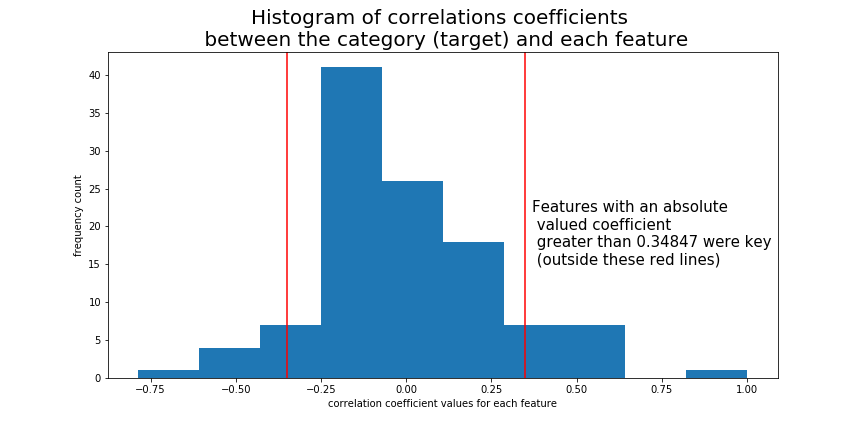
Once the data was in binary form, a histogram plot between the correlation of each feature and the class (the target) was made. Using the values of the correlations, a trial and error process was done by fitting an assortment of classification models to a set of features that had a magnitude (absolute value) greater than a threshold correlation value. It was found that all the set of features with a magnitude greater than abs(±0.34847) was enough data to produce a model that performed with perfect accuracy on a 70-30 train test split. There were 19 features (out of 112) that met this criteria.
.
Feature Ranking
After converting into binary form, features were then fed into the models and ranked descendingly in accordance to the magnitude of their correlation coefficient with the target variable, class. Thus the first feature fed into the model had the highest magnitude of correlation, the second had the second highest, and so on. The first five rows of the feature rank table looked like this;
| Rank | Feature | Correlation with target |
|---|---|---|
| 1 | odor_n | -0.7855566222367798 |
| 2 | odor_f | 0.6238419598140276 |
| 3 | stalk-surface-above-ring_k | 0.587658257630713 |
| 4 | stalk-surface-below-ring_k | 0.5735240117095786 |
| 5 | ring-type_p | -0.5404689127748091 |
And so on, upto all 112 engineered features. The 19 most important features will be discussed below.
A for loop was designed to feed the five different models sets of data features in order of their correlation rank. So at the first iteration the models were fitted and evaluated on the first feature odor_n, in the second iteration the models were fitted and evaluated on the first two features (odor_n and odor_f), the third iteration used the first three features (ordor_n,odor_f,stalk-surface-above-ring_k), and so on.
Hence the loop to build the models went as such;
for indices in feature_ranks.index:
    models.fit(data[feature_ranks['Feature'].loc[:indices]],data['class'])
    models.predict(data[feature_ranks['Feature'].loc[:indices]],data['class'])
    evaluate models, etc.
III. Model Selection
Multiple models were chosen for evaluation. These included:
- logistic regression
- K-nearest-neighbors
- support vector machine
- decision tree classifier
- random forest classifier
Model performance was evaluated on:
- Accuracy score
- F1 score
- The minimum number of features needed to achieve the models highest metrics
- Combined time of training plus predicting
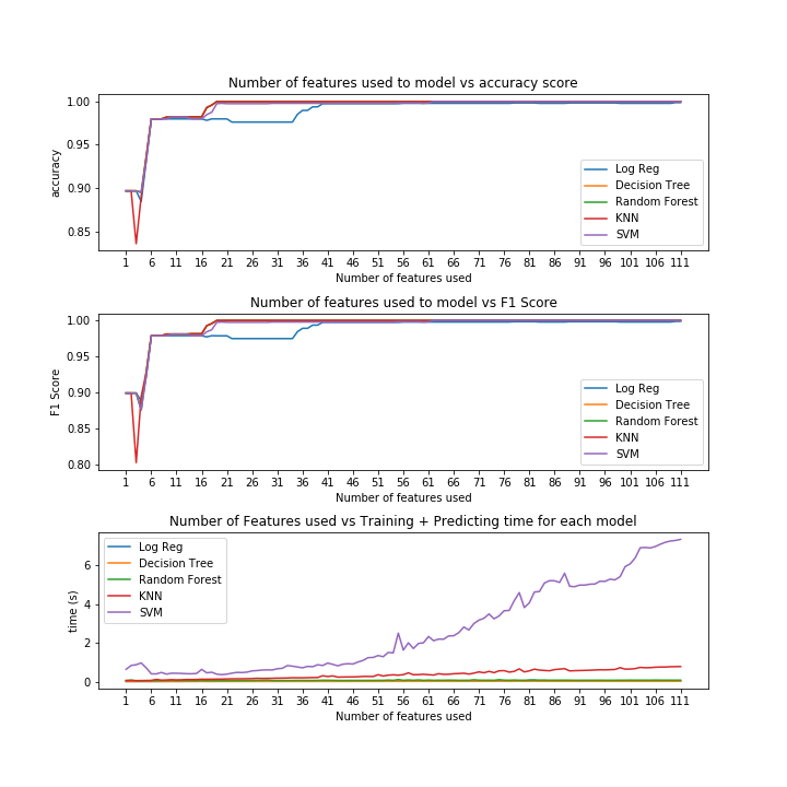
Each model was fed through the previously mentioned for-loop and evaluated on a 70-30 train test split. As we can see from the graphs below, it was the top 19 ranked features that most of the models began to score with perfect accuracy.
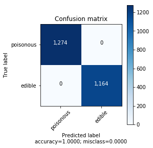
Despite random forest, k-nearest-neighbors and decision trees all getting perfect scores when fed 19 features, it was decision trees which performed in the shortest amount time. Thus, decision tree classifier was the best model.
IV. Model Evaluation: Decision Tree Classifier
Decision tree classifier was the model which met the criteria of the performing in the least amount of time, with the least number of features and having maximum performance metrics on F1 and accuracy scores.
| Metric | Value |
|---|---|
| Accuracy | 1.0000 |
| F1 score | 1.0000 |
| AUC | 1.0000 |
| Number of features used | 19 out of 112 |
| train+predict time | 0.006112(s) |
| Test set size | 2438 (30%) |
| Train set size | 5686 (70%) |
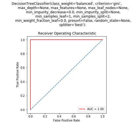
Specifically, the hyperparameters and roc-auc curve were;
Comments on perfect accuracy metrics
Though its not common to get perfect scores on models, it does happen. Moreover, it was quite obvious that many other who have worked with this data set on the kaggle competition achieved perfect scoring metrics as well.
V.Conclusions
Using only 19 pieces of information, we can conclude with 100% certainty that a mushroom is edible or poisonous. These are the 19 features, ranked in descending order by the absolute value with their correlation with the target, class. Recall that in the target class, edible was marked as 0 and poisonous was marked at 1.
A negative correlation means if a mushroom has that feature it is more likely to be edible
A positive correlation means if a mushroom has that feature it is more likely to be poisonous.
| Rank | Feature | Correlation with target |
|---|---|---|
| 1 | odor_n | -0.7855566222367798 |
| 2 | odor_f | 0.6238419598140276 |
| 3 | stalk-surface-above-ring_k | 0.587658257630713 |
| 4 | stalk-surface-below-ring_k | 0.5735240117095786 |
| 5 | ring-type_p | -0.5404689127748091 |
| 6 | gill-size_n | 0.5400243574329782 |
| 7 | gill-size_b | -0.5400243574329637 |
| 8 | gill-color_b | 0.5388081615534243 |
| 9 | bruises_f | 0.5015303774076804 |
| 10 | bruises_t | -0.5015303774076804 |
| 11 | stalk-surface-above-ring_s | -0.49131418071172045 |
| 12 | spore-print-color_h | 0.49022917056952875 |
| 13 | ring-type_l | 0.4516190663173296 |
| 14 | population_v | 0.44372237905537937 |
| 15 | stalk-surface-below-ring_s | -0.42544404585499374 |
| 16 | spore-print-color_n | -0.41664529710731296 |
| 17 | spore-print-color_k | -0.3968322009032092 |
| 18 | spore-print-color_w | 0.3573840060325314 |
| 19 | gill-spacing_c | 0.34838678518425714 |
Out original features (before engineering), the 19 listed above were engineered from 9 of the 22 originals. They were as follows;
| Rank | Feature |
|---|---|
| 1 | Odor |
| 2 | Stalk-surface-above-ring |
| 3 | Stalk-surface-below-ring |
| 4 | Ring type |
| 5 | Gill size |
| 6 | Bruises |
| 7 | Spore-print-color |
| 8 | population |
| 9 | Gill-spacing |
Interpreting these features
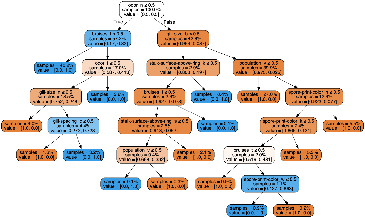
The decision tree model has a workflow which helps us draw conclusions.
Starting at the top, for a given row (i.e. a given mushroom) if the feature odor_n <=0.5 (which really means odor_n = 0 or odor_none=False, or it has an odor) AND it bruises_t <=0.5 (i.e. bruises_t = 0 or, the mushroom does NOT bruise), then we conclude the mushroom is poisonous. More conclusions can be made simply by following the tree.
VI.References
Links to my codeded notebooks to build the project
Links/other sources