Teaching regression: A basic tutorial on how to build a regression model from start to finish
By Joe Ganser
I.Introduction
In this notebook, I will be creating a simple work flow tutorial that allows beginner data science students to go through the process of building a regression model. This is for students who have completed most of my introduction to data science class and have basic familiarity with data science.
Background info
The data set we'll be working with is well known and studied. It describes real-estate sales on houses in AMES Iowa, and the target variable we're trying to predict is the price of a home. Lets load the data and begin exploring. A lot of kaggle projects have been made from it, and you can find them here.
II.Exploratory Data Analysis
In any data science project, we always start of by getting a good glimpse of what kind of data we're looking at. This is called "exploratory data analysis" (EDA). There are a few things we need to look at at our first round of EDA:
- The number of rows/columns.
- The data types on each columns.
- Get the min, max, mean values of each column
- The number of missing values.
Lets start by loading the dataset, and observing it's dimensions. Our target variable y is the house price, and the rest of the variables (X) are our predictors. We want to load the file train.csv because it will train our models.
Now split the data set into a predictor table (X) and a target table y
Now look at the head of the predictor table, and print it's shape.
(1460, 80)
| Id | MSSubClass | MSZoning | LotFrontage | LotArea | Street | Alley | LotShape | LandContour | Utilities | LotConfig | LandSlope | Neighborhood | Condition1 | Condition2 | BldgType | HouseStyle | OverallQual | OverallCond | YearBuilt | YearRemodAdd | RoofStyle | RoofMatl | Exterior1st | Exterior2nd | MasVnrType | MasVnrArea | ExterQual | ExterCond | Foundation | BsmtQual | BsmtCond | BsmtExposure | BsmtFinType1 | BsmtFinSF1 | BsmtFinType2 | BsmtFinSF2 | BsmtUnfSF | TotalBsmtSF | Heating | HeatingQC | CentralAir | Electrical | 1stFlrSF | 2ndFlrSF | LowQualFinSF | GrLivArea | BsmtFullBath | BsmtHalfBath | FullBath | HalfBath | BedroomAbvGr | KitchenAbvGr | KitchenQual | TotRmsAbvGrd | Functional | Fireplaces | FireplaceQu | GarageType | GarageYrBlt | GarageFinish | GarageCars | GarageArea | GarageQual | GarageCond | PavedDrive | WoodDeckSF | OpenPorchSF | EnclosedPorch | 3SsnPorch | ScreenPorch | PoolArea | PoolQC | Fence | MiscFeature | MiscVal | MoSold | YrSold | SaleType | SaleCondition |
|---|---|---|---|---|---|---|---|---|---|---|---|---|---|---|---|---|---|---|---|---|---|---|---|---|---|---|---|---|---|---|---|---|---|---|---|---|---|---|---|---|---|---|---|---|---|---|---|---|---|---|---|---|---|---|---|---|---|---|---|---|---|---|---|---|---|---|---|---|---|---|---|---|---|---|---|---|---|---|---|
| 1 | 60 | RL | 65.0 | 8450 | Pave | Reg | Lvl | AllPub | Inside | Gtl | CollgCr | Norm | Norm | 1Fam | 2Story | 7 | 5 | 2003 | 2003 | Gable | CompShg | VinylSd | VinylSd | BrkFace | 196.0 | Gd | TA | PConc | Gd | TA | No | GLQ | 706 | Unf | 0 | 150 | 856 | GasA | Ex | Y | SBrkr | 856 | 854 | 0 | 1710 | 1 | 0 | 2 | 1 | 3 | 1 | Gd | 8 | Typ | 0 | Attchd | 2003.0 | RFn | 2 | 548 | TA | TA | Y | 0 | 61 | 0 | 0 | 0 | 0 | 0 | 2 | 2008 | WD | Normal | |||||
| 2 | 20 | RL | 80.0 | 9600 | Pave | Reg | Lvl | AllPub | FR2 | Gtl | Veenker | Feedr | Norm | 1Fam | 1Story | 6 | 8 | 1976 | 1976 | Gable | CompShg | MetalSd | MetalSd | None | 0.0 | TA | TA | CBlock | Gd | TA | Gd | ALQ | 978 | Unf | 0 | 284 | 1262 | GasA | Ex | Y | SBrkr | 1262 | 0 | 0 | 1262 | 0 | 1 | 2 | 0 | 3 | 1 | TA | 6 | Typ | 1 | TA | Attchd | 1976.0 | RFn | 2 | 460 | TA | TA | Y | 298 | 0 | 0 | 0 | 0 | 0 | 0 | 5 | 2007 | WD | Normal | ||||
| 3 | 60 | RL | 68.0 | 11250 | Pave | IR1 | Lvl | AllPub | Inside | Gtl | CollgCr | Norm | Norm | 1Fam | 2Story | 7 | 5 | 2001 | 2002 | Gable | CompShg | VinylSd | VinylSd | BrkFace | 162.0 | Gd | TA | PConc | Gd | TA | Mn | GLQ | 486 | Unf | 0 | 434 | 920 | GasA | Ex | Y | SBrkr | 920 | 866 | 0 | 1786 | 1 | 0 | 2 | 1 | 3 | 1 | Gd | 6 | Typ | 1 | TA | Attchd | 2001.0 | RFn | 2 | 608 | TA | TA | Y | 0 | 42 | 0 | 0 | 0 | 0 | 0 | 9 | 2008 | WD | Normal | ||||
| 4 | 70 | RL | 60.0 | 9550 | Pave | IR1 | Lvl | AllPub | Corner | Gtl | Crawfor | Norm | Norm | 1Fam | 2Story | 7 | 5 | 1915 | 1970 | Gable | CompShg | Wd Sdng | Wd Shng | None | 0.0 | TA | TA | BrkTil | TA | Gd | No | ALQ | 216 | Unf | 0 | 540 | 756 | GasA | Gd | Y | SBrkr | 961 | 756 | 0 | 1717 | 1 | 0 | 1 | 0 | 3 | 1 | Gd | 7 | Typ | 1 | Gd | Detchd | 1998.0 | Unf | 3 | 642 | TA | TA | Y | 0 | 35 | 272 | 0 | 0 | 0 | 0 | 2 | 2006 | WD | Abnorml | ||||
| 5 | 60 | RL | 84.0 | 14260 | Pave | IR1 | Lvl | AllPub | FR2 | Gtl | NoRidge | Norm | Norm | 1Fam | 2Story | 8 | 5 | 2000 | 2000 | Gable | CompShg | VinylSd | VinylSd | BrkFace | 350.0 | Gd | TA | PConc | Gd | TA | Av | GLQ | 655 | Unf | 0 | 490 | 1145 | GasA | Ex | Y | SBrkr | 1145 | 1053 | 0 | 2198 | 1 | 0 | 2 | 1 | 4 | 1 | Gd | 9 | Typ | 1 | TA | Attchd | 2000.0 | RFn | 3 | 836 | TA | TA | Y | 192 | 84 | 0 | 0 | 0 | 0 | 0 | 12 | 2008 | WD | Normal |
Now use the .info() method to find that datatypes on all of the columns (including the target!)
<class 'pandas.core.frame.DataFrame'>
RangeIndex: 1460 entries, 0 to 1459
Data columns (total 81 columns):
Id               1460 non-null int64
MSSubClass       1460 non-null int64
MSZoning         1460 non-null object
LotFrontage      1201 non-null float64
LotArea          1460 non-null int64
Street           1460 non-null object
Alley            91 non-null object
LotShape         1460 non-null object
LandContour      1460 non-null object
Utilities        1460 non-null object
LotConfig        1460 non-null object
LandSlope        1460 non-null object
Neighborhood     1460 non-null object
Condition1       1460 non-null object
Condition2       1460 non-null object
BldgType         1460 non-null object
HouseStyle       1460 non-null object
OverallQual      1460 non-null int64
OverallCond      1460 non-null int64
YearBuilt        1460 non-null int64
YearRemodAdd     1460 non-null int64
RoofStyle        1460 non-null object
RoofMatl         1460 non-null object
Exterior1st      1460 non-null object
Exterior2nd      1460 non-null object
MasVnrType       1452 non-null object
MasVnrArea       1452 non-null float64
ExterQual        1460 non-null object
ExterCond        1460 non-null object
Foundation       1460 non-null object
BsmtQual         1423 non-null object
BsmtCond         1423 non-null object
BsmtExposure     1422 non-null object
BsmtFinType1     1423 non-null object
BsmtFinSF1       1460 non-null int64
BsmtFinType2     1422 non-null object
BsmtFinSF2       1460 non-null int64
BsmtUnfSF        1460 non-null int64
TotalBsmtSF      1460 non-null int64
Heating          1460 non-null object
HeatingQC        1460 non-null object
CentralAir       1460 non-null object
Electrical       1459 non-null object
1stFlrSF         1460 non-null int64
2ndFlrSF         1460 non-null int64
LowQualFinSF     1460 non-null int64
GrLivArea        1460 non-null int64
BsmtFullBath     1460 non-null int64
BsmtHalfBath     1460 non-null int64
FullBath         1460 non-null int64
HalfBath         1460 non-null int64
BedroomAbvGr     1460 non-null int64
KitchenAbvGr     1460 non-null int64
KitchenQual      1460 non-null object
TotRmsAbvGrd     1460 non-null int64
Functional       1460 non-null object
Fireplaces       1460 non-null int64
FireplaceQu      770 non-null object
GarageType       1379 non-null object
GarageYrBlt      1379 non-null float64
GarageFinish     1379 non-null object
GarageCars       1460 non-null int64
GarageArea       1460 non-null int64
GarageQual       1379 non-null object
GarageCond       1379 non-null object
PavedDrive       1460 non-null object
WoodDeckSF       1460 non-null int64
OpenPorchSF      1460 non-null int64
EnclosedPorch    1460 non-null int64
3SsnPorch        1460 non-null int64
ScreenPorch      1460 non-null int64
PoolArea         1460 non-null int64
PoolQC           7 non-null object
Fence            281 non-null object
MiscFeature      54 non-null object
MiscVal          1460 non-null int64
MoSold           1460 non-null int64
YrSold           1460 non-null int64
SaleType         1460 non-null object
SaleCondition    1460 non-null object
SalePrice        1460 non-null int64
dtypes: float64(3), int64(35), object(43)
memory usage: 924.0+ KB
Now use the .describe() method on the full data set to get the min,max,mean and other values for each column. Try adding in the .transpose() method to make it a little more readable.
| count | mean | std | min | 25% | 50% | 75% | max |
|---|---|---|---|---|---|---|---|
| 1460.0 | 730.5 | 421.6100093688479 | 1.0 | 365.75 | 730.5 | 1095.25 | 1460.0 |
| 1460.0 | 56.897260273972606 | 42.30057099381035 | 20.0 | 20.0 | 50.0 | 70.0 | 190.0 |
| 1201.0 | 70.04995836802665 | 24.284751774483183 | 21.0 | 59.0 | 69.0 | 80.0 | 313.0 |
| 1460.0 | 10516.828082191782 | 9981.264932379147 | 1300.0 | 7553.5 | 9478.5 | 11601.5 | 215245.0 |
| 1460.0 | 6.0993150684931505 | 1.3829965467415923 | 1.0 | 5.0 | 6.0 | 7.0 | 10.0 |
| 1460.0 | 5.575342465753424 | 1.1127993367127367 | 1.0 | 5.0 | 5.0 | 6.0 | 9.0 |
| 1460.0 | 1971.267808219178 | 30.202904042525265 | 1872.0 | 1954.0 | 1973.0 | 2000.0 | 2010.0 |
| 1460.0 | 1984.8657534246574 | 20.645406807709396 | 1950.0 | 1967.0 | 1994.0 | 2004.0 | 2010.0 |
| 1452.0 | 103.68526170798899 | 181.06620658721818 | 0.0 | 0.0 | 0.0 | 166.0 | 1600.0 |
| 1460.0 | 443.6397260273973 | 456.09809084092456 | 0.0 | 0.0 | 383.5 | 712.25 | 5644.0 |
| 1460.0 | 46.54931506849315 | 161.31927280654057 | 0.0 | 0.0 | 0.0 | 0.0 | 1474.0 |
| 1460.0 | 567.2404109589041 | 441.8669552924342 | 0.0 | 223.0 | 477.5 | 808.0 | 2336.0 |
| 1460.0 | 1057.4294520547944 | 438.7053244594705 | 0.0 | 795.75 | 991.5 | 1298.25 | 6110.0 |
| 1460.0 | 1162.626712328767 | 386.5877380410738 | 334.0 | 882.0 | 1087.0 | 1391.25 | 4692.0 |
| 1460.0 | 346.99246575342465 | 436.5284358862591 | 0.0 | 0.0 | 0.0 | 728.0 | 2065.0 |
| 1460.0 | 5.844520547945206 | 48.623081433519125 | 0.0 | 0.0 | 0.0 | 0.0 | 572.0 |
| 1460.0 | 1515.463698630137 | 525.4803834232027 | 334.0 | 1129.5 | 1464.0 | 1776.75 | 5642.0 |
| 1460.0 | 0.42534246575342466 | 0.5189106060897992 | 0.0 | 0.0 | 0.0 | 1.0 | 3.0 |
| 1460.0 | 0.057534246575342465 | 0.23875264627920764 | 0.0 | 0.0 | 0.0 | 0.0 | 2.0 |
| 1460.0 | 1.5650684931506849 | 0.5509158012954318 | 0.0 | 1.0 | 2.0 | 2.0 | 3.0 |
| 1460.0 | 0.38287671232876713 | 0.5028853810928973 | 0.0 | 0.0 | 0.0 | 1.0 | 2.0 |
| 1460.0 | 2.8664383561643834 | 0.8157780441442212 | 0.0 | 2.0 | 3.0 | 3.0 | 8.0 |
| 1460.0 | 1.0465753424657533 | 0.22033819838402977 | 0.0 | 1.0 | 1.0 | 1.0 | 3.0 |
| 1460.0 | 6.517808219178082 | 1.625393290584064 | 2.0 | 5.0 | 6.0 | 7.0 | 14.0 |
| 1460.0 | 0.613013698630137 | 0.6446663863122344 | 0.0 | 0.0 | 1.0 | 1.0 | 3.0 |
| 1379.0 | 1978.5061638868744 | 24.689724768590214 | 1900.0 | 1961.0 | 1980.0 | 2002.0 | 2010.0 |
| 1460.0 | 1.7671232876712328 | 0.7473150101111116 | 0.0 | 1.0 | 2.0 | 2.0 | 4.0 |
| 1460.0 | 472.9801369863014 | 213.80484145338076 | 0.0 | 334.5 | 480.0 | 576.0 | 1418.0 |
| 1460.0 | 94.2445205479452 | 125.33879435172359 | 0.0 | 0.0 | 0.0 | 168.0 | 857.0 |
| 1460.0 | 46.66027397260274 | 66.25602767664974 | 0.0 | 0.0 | 25.0 | 68.0 | 547.0 |
| 1460.0 | 21.954109589041096 | 61.11914860172879 | 0.0 | 0.0 | 0.0 | 0.0 | 552.0 |
| 1460.0 | 3.4095890410958902 | 29.317330556782203 | 0.0 | 0.0 | 0.0 | 0.0 | 508.0 |
| 1460.0 | 15.060958904109588 | 55.757415281874486 | 0.0 | 0.0 | 0.0 | 0.0 | 480.0 |
| 1460.0 | 2.758904109589041 | 40.17730694453043 | 0.0 | 0.0 | 0.0 | 0.0 | 738.0 |
| 1460.0 | 43.489041095890414 | 496.1230244579311 | 0.0 | 0.0 | 0.0 | 0.0 | 15500.0 |
| 1460.0 | 6.321917808219178 | 2.7036262083595197 | 1.0 | 5.0 | 6.0 | 8.0 | 12.0 |
| 1460.0 | 2007.8157534246575 | 1.328095120552104 | 2006.0 | 2007.0 | 2008.0 | 2009.0 | 2010.0 |
| 1460.0 | 180921.19589041095 | 79442.50288288663 | 34900.0 | 129975.0 | 163000.0 | 214000.0 | 755000.0 |
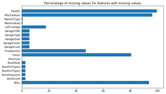
Now lets code up a script to create a bar chart that counts the number of missing values in each of the predictor columns. Intutively, we could suggest that a feature with a lot of missing values might not be important. This may or may not be true, but it's important to know what is and isn't there to begin with.
III.Feature engineering & Data Cleaning
Cleaning data and manipulating features is a major part of any project. In this part of a data science project we solve problems such as:
- Turning categorical (string) variables into numerical ones
- Dealing with missing values by changing them or removing them
- Dealing with outliers by changing them or removing them
- Make corrections to data types so machine learning algorithms can read them; e.g. removing a dollar sign to conver
'$4.51'to4.51so it's a float - Grouping columns of different data types to be dealt with differently
First, lets seperate the numerical predictors from the cateogircal (string) ones. Do this by going through the list of columns and selecting those with .dtypes(column)=='object' for categorical, and not equal for numerical.
Now lets look at the categorical features. Print the shape and display the head of the table.
(1460, 43)
| MSZoning | Street | Alley | LotShape | LandContour | Utilities | LotConfig | LandSlope | Neighborhood | Condition1 | Condition2 | BldgType | HouseStyle | RoofStyle | RoofMatl | Exterior1st | Exterior2nd | MasVnrType | ExterQual | ExterCond | Foundation | BsmtQual | BsmtCond | BsmtExposure | BsmtFinType1 | BsmtFinType2 | Heating | HeatingQC | CentralAir | Electrical | KitchenQual | Functional | FireplaceQu | GarageType | GarageFinish | GarageQual | GarageCond | PavedDrive | PoolQC | Fence | MiscFeature | SaleType | SaleCondition |
|---|---|---|---|---|---|---|---|---|---|---|---|---|---|---|---|---|---|---|---|---|---|---|---|---|---|---|---|---|---|---|---|---|---|---|---|---|---|---|---|---|---|---|
| RL | Pave | Reg | Lvl | AllPub | Inside | Gtl | CollgCr | Norm | Norm | 1Fam | 2Story | Gable | CompShg | VinylSd | VinylSd | BrkFace | Gd | TA | PConc | Gd | TA | No | GLQ | Unf | GasA | Ex | Y | SBrkr | Gd | Typ | Attchd | RFn | TA | TA | Y | WD | Normal | |||||
| RL | Pave | Reg | Lvl | AllPub | FR2 | Gtl | Veenker | Feedr | Norm | 1Fam | 1Story | Gable | CompShg | MetalSd | MetalSd | None | TA | TA | CBlock | Gd | TA | Gd | ALQ | Unf | GasA | Ex | Y | SBrkr | TA | Typ | TA | Attchd | RFn | TA | TA | Y | WD | Normal | ||||
| RL | Pave | IR1 | Lvl | AllPub | Inside | Gtl | CollgCr | Norm | Norm | 1Fam | 2Story | Gable | CompShg | VinylSd | VinylSd | BrkFace | Gd | TA | PConc | Gd | TA | Mn | GLQ | Unf | GasA | Ex | Y | SBrkr | Gd | Typ | TA | Attchd | RFn | TA | TA | Y | WD | Normal | ||||
| RL | Pave | IR1 | Lvl | AllPub | Corner | Gtl | Crawfor | Norm | Norm | 1Fam | 2Story | Gable | CompShg | Wd Sdng | Wd Shng | None | TA | TA | BrkTil | TA | Gd | No | ALQ | Unf | GasA | Gd | Y | SBrkr | Gd | Typ | Gd | Detchd | Unf | TA | TA | Y | WD | Abnorml | ||||
| RL | Pave | IR1 | Lvl | AllPub | FR2 | Gtl | NoRidge | Norm | Norm | 1Fam | 2Story | Gable | CompShg | VinylSd | VinylSd | BrkFace | Gd | TA | PConc | Gd | TA | Av | GLQ | Unf | GasA | Ex | Y | SBrkr | Gd | Typ | TA | Attchd | RFn | TA | TA | Y | WD | Normal |
Now we have to convert this categorical data into numerical data. This is done using the pandas .get_dummies(data) function, which basically makes a new column for each categorical variable in a given column, and puts a value of 1 if that category is present for that row. The down side of doing this is the number of variables then blows up, which we will deal with later during feature selection.
Acting on the original table df, we get dummies of the categories, drop the categories from the table df and then concatenate the dummies to table df. This will lead us with only numbers in our dataframe, no strings.
If you did it right you should now have 290 columns.
| Id | MSSubClass | LotFrontage | LotArea | OverallQual | OverallCond | YearBuilt | YearRemodAdd | MasVnrArea | BsmtFinSF1 | BsmtFinSF2 | BsmtUnfSF | TotalBsmtSF | 1stFlrSF | 2ndFlrSF | LowQualFinSF | GrLivArea | BsmtFullBath | BsmtHalfBath | FullBath | HalfBath | BedroomAbvGr | KitchenAbvGr | TotRmsAbvGrd | Fireplaces | GarageYrBlt | GarageCars | GarageArea | WoodDeckSF | OpenPorchSF | EnclosedPorch | 3SsnPorch | ScreenPorch | PoolArea | MiscVal | MoSold | YrSold | SalePrice | MSZoning_C (all) | MSZoning_FV | MSZoning_RH | MSZoning_RL | MSZoning_RM | Street_Grvl | Street_Pave | Alley_Grvl | Alley_Pave | LotShape_IR1 | LotShape_IR2 | LotShape_IR3 | LotShape_Reg | LandContour_Bnk | LandContour_HLS | LandContour_Low | LandContour_Lvl | Utilities_AllPub | Utilities_NoSeWa | LotConfig_Corner | LotConfig_CulDSac | LotConfig_FR2 | LotConfig_FR3 | LotConfig_Inside | LandSlope_Gtl | LandSlope_Mod | LandSlope_Sev | Neighborhood_Blmngtn | Neighborhood_Blueste | Neighborhood_BrDale | Neighborhood_BrkSide | Neighborhood_ClearCr | Neighborhood_CollgCr | Neighborhood_Crawfor | Neighborhood_Edwards | Neighborhood_Gilbert | Neighborhood_IDOTRR | Neighborhood_MeadowV | Neighborhood_Mitchel | Neighborhood_NAmes | Neighborhood_NPkVill | Neighborhood_NWAmes | Neighborhood_NoRidge | Neighborhood_NridgHt | Neighborhood_OldTown | Neighborhood_SWISU | Neighborhood_Sawyer | Neighborhood_SawyerW | Neighborhood_Somerst | Neighborhood_StoneBr | Neighborhood_Timber | Neighborhood_Veenker | Condition1_Artery | Condition1_Feedr | Condition1_Norm | Condition1_PosA | Condition1_PosN | Condition1_RRAe | Condition1_RRAn | Condition1_RRNe | Condition1_RRNn | Condition2_Artery | Condition2_Feedr | Condition2_Norm | Condition2_PosA | Condition2_PosN | Condition2_RRAe | Condition2_RRAn | Condition2_RRNn | BldgType_1Fam | BldgType_2fmCon | BldgType_Duplex | BldgType_Twnhs | BldgType_TwnhsE | HouseStyle_1.5Fin | HouseStyle_1.5Unf | HouseStyle_1Story | HouseStyle_2.5Fin | HouseStyle_2.5Unf | HouseStyle_2Story | HouseStyle_SFoyer | HouseStyle_SLvl | RoofStyle_Flat | RoofStyle_Gable | RoofStyle_Gambrel | RoofStyle_Hip | RoofStyle_Mansard | RoofStyle_Shed | RoofMatl_ClyTile | RoofMatl_CompShg | RoofMatl_Membran | RoofMatl_Metal | RoofMatl_Roll | RoofMatl_Tar&Grv | RoofMatl_WdShake | RoofMatl_WdShngl | Exterior1st_AsbShng | Exterior1st_AsphShn | Exterior1st_BrkComm | Exterior1st_BrkFace | Exterior1st_CBlock | Exterior1st_CemntBd | Exterior1st_HdBoard | Exterior1st_ImStucc | Exterior1st_MetalSd | Exterior1st_Plywood | Exterior1st_Stone | Exterior1st_Stucco | Exterior1st_VinylSd | Exterior1st_Wd Sdng | Exterior1st_WdShing | Exterior2nd_AsbShng | Exterior2nd_AsphShn | Exterior2nd_Brk Cmn | Exterior2nd_BrkFace | Exterior2nd_CBlock | Exterior2nd_CmentBd | Exterior2nd_HdBoard | Exterior2nd_ImStucc | Exterior2nd_MetalSd | Exterior2nd_Other | Exterior2nd_Plywood | Exterior2nd_Stone | Exterior2nd_Stucco | Exterior2nd_VinylSd | Exterior2nd_Wd Sdng | Exterior2nd_Wd Shng | MasVnrType_BrkCmn | MasVnrType_BrkFace | MasVnrType_None | MasVnrType_Stone | ExterQual_Ex | ExterQual_Fa | ExterQual_Gd | ExterQual_TA | ExterCond_Ex | ExterCond_Fa | ExterCond_Gd | ExterCond_Po | ExterCond_TA | Foundation_BrkTil | Foundation_CBlock | Foundation_PConc | Foundation_Slab | Foundation_Stone | Foundation_Wood | BsmtQual_Ex | BsmtQual_Fa | BsmtQual_Gd | BsmtQual_TA | BsmtCond_Fa | BsmtCond_Gd | BsmtCond_Po | BsmtCond_TA | BsmtExposure_Av | BsmtExposure_Gd | BsmtExposure_Mn | BsmtExposure_No | BsmtFinType1_ALQ | BsmtFinType1_BLQ | BsmtFinType1_GLQ | BsmtFinType1_LwQ | BsmtFinType1_Rec | BsmtFinType1_Unf | BsmtFinType2_ALQ | BsmtFinType2_BLQ | BsmtFinType2_GLQ | BsmtFinType2_LwQ | BsmtFinType2_Rec | BsmtFinType2_Unf | Heating_Floor | Heating_GasA | Heating_GasW | Heating_Grav | Heating_OthW | Heating_Wall | HeatingQC_Ex | HeatingQC_Fa | HeatingQC_Gd | HeatingQC_Po | HeatingQC_TA | CentralAir_N | CentralAir_Y | Electrical_FuseA | Electrical_FuseF | Electrical_FuseP | Electrical_Mix | Electrical_SBrkr | KitchenQual_Ex | KitchenQual_Fa | KitchenQual_Gd | KitchenQual_TA | Functional_Maj1 | Functional_Maj2 | Functional_Min1 | Functional_Min2 | Functional_Mod | Functional_Sev | Functional_Typ | FireplaceQu_Ex | FireplaceQu_Fa | FireplaceQu_Gd | FireplaceQu_Po | FireplaceQu_TA | GarageType_2Types | GarageType_Attchd | GarageType_Basment | GarageType_BuiltIn | GarageType_CarPort | GarageType_Detchd | GarageFinish_Fin | GarageFinish_RFn | GarageFinish_Unf | GarageQual_Ex | GarageQual_Fa | GarageQual_Gd | GarageQual_Po | GarageQual_TA | GarageCond_Ex | GarageCond_Fa | GarageCond_Gd | GarageCond_Po | GarageCond_TA | PavedDrive_N | PavedDrive_P | PavedDrive_Y | PoolQC_Ex | PoolQC_Fa | PoolQC_Gd | Fence_GdPrv | Fence_GdWo | Fence_MnPrv | Fence_MnWw | MiscFeature_Gar2 | MiscFeature_Othr | MiscFeature_Shed | MiscFeature_TenC | SaleType_COD | SaleType_CWD | SaleType_Con | SaleType_ConLD | SaleType_ConLI | SaleType_ConLw | SaleType_New | SaleType_Oth | SaleType_WD | SaleCondition_Abnorml | SaleCondition_AdjLand | SaleCondition_Alloca | SaleCondition_Family | SaleCondition_Normal | SaleCondition_Partial |
|---|---|---|---|---|---|---|---|---|---|---|---|---|---|---|---|---|---|---|---|---|---|---|---|---|---|---|---|---|---|---|---|---|---|---|---|---|---|---|---|---|---|---|---|---|---|---|---|---|---|---|---|---|---|---|---|---|---|---|---|---|---|---|---|---|---|---|---|---|---|---|---|---|---|---|---|---|---|---|---|---|---|---|---|---|---|---|---|---|---|---|---|---|---|---|---|---|---|---|---|---|---|---|---|---|---|---|---|---|---|---|---|---|---|---|---|---|---|---|---|---|---|---|---|---|---|---|---|---|---|---|---|---|---|---|---|---|---|---|---|---|---|---|---|---|---|---|---|---|---|---|---|---|---|---|---|---|---|---|---|---|---|---|---|---|---|---|---|---|---|---|---|---|---|---|---|---|---|---|---|---|---|---|---|---|---|---|---|---|---|---|---|---|---|---|---|---|---|---|---|---|---|---|---|---|---|---|---|---|---|---|---|---|---|---|---|---|---|---|---|---|---|---|---|---|---|---|---|---|---|---|---|---|---|---|---|---|---|---|---|---|---|---|---|---|---|---|---|---|---|---|---|---|---|---|---|---|---|---|---|---|---|---|---|---|---|---|---|---|---|---|---|---|---|---|---|---|---|---|---|---|---|---|---|---|---|---|---|---|---|
| 1 | 60 | 65.0 | 8450 | 7 | 5 | 2003 | 2003 | 196.0 | 706 | 0 | 150 | 856 | 856 | 854 | 0 | 1710 | 1 | 0 | 2 | 1 | 3 | 1 | 8 | 0 | 2003.0 | 2 | 548 | 0 | 61 | 0 | 0 | 0 | 0 | 0 | 2 | 2008 | 208500 | 0 | 0 | 0 | 1 | 0 | 0 | 1 | 0 | 0 | 0 | 0 | 0 | 1 | 0 | 0 | 0 | 1 | 1 | 0 | 0 | 0 | 0 | 0 | 1 | 1 | 0 | 0 | 0 | 0 | 0 | 0 | 0 | 1 | 0 | 0 | 0 | 0 | 0 | 0 | 0 | 0 | 0 | 0 | 0 | 0 | 0 | 0 | 0 | 0 | 0 | 0 | 0 | 0 | 0 | 1 | 0 | 0 | 0 | 0 | 0 | 0 | 0 | 0 | 1 | 0 | 0 | 0 | 0 | 0 | 1 | 0 | 0 | 0 | 0 | 0 | 0 | 0 | 0 | 0 | 1 | 0 | 0 | 0 | 1 | 0 | 0 | 0 | 0 | 0 | 1 | 0 | 0 | 0 | 0 | 0 | 0 | 0 | 0 | 0 | 0 | 0 | 0 | 0 | 0 | 0 | 0 | 0 | 0 | 1 | 0 | 0 | 0 | 0 | 0 | 0 | 0 | 0 | 0 | 0 | 0 | 0 | 0 | 0 | 0 | 1 | 0 | 0 | 0 | 1 | 0 | 0 | 0 | 0 | 1 | 0 | 0 | 0 | 0 | 0 | 1 | 0 | 0 | 1 | 0 | 0 | 0 | 0 | 0 | 1 | 0 | 0 | 0 | 0 | 1 | 0 | 0 | 0 | 1 | 0 | 0 | 1 | 0 | 0 | 0 | 0 | 0 | 0 | 0 | 0 | 1 | 0 | 1 | 0 | 0 | 0 | 0 | 1 | 0 | 0 | 0 | 0 | 0 | 1 | 0 | 0 | 0 | 0 | 1 | 0 | 0 | 1 | 0 | 0 | 0 | 0 | 0 | 0 | 0 | 1 | 0 | 0 | 0 | 0 | 0 | 0 | 1 | 0 | 0 | 0 | 0 | 0 | 1 | 0 | 0 | 0 | 0 | 0 | 1 | 0 | 0 | 0 | 0 | 1 | 0 | 0 | 1 | 0 | 0 | 0 | 0 | 0 | 0 | 0 | 0 | 0 | 0 | 0 | 0 | 0 | 0 | 0 | 0 | 0 | 0 | 0 | 1 | 0 | 0 | 0 | 0 | 1 | 0 |
| 2 | 20 | 80.0 | 9600 | 6 | 8 | 1976 | 1976 | 0.0 | 978 | 0 | 284 | 1262 | 1262 | 0 | 0 | 1262 | 0 | 1 | 2 | 0 | 3 | 1 | 6 | 1 | 1976.0 | 2 | 460 | 298 | 0 | 0 | 0 | 0 | 0 | 0 | 5 | 2007 | 181500 | 0 | 0 | 0 | 1 | 0 | 0 | 1 | 0 | 0 | 0 | 0 | 0 | 1 | 0 | 0 | 0 | 1 | 1 | 0 | 0 | 0 | 1 | 0 | 0 | 1 | 0 | 0 | 0 | 0 | 0 | 0 | 0 | 0 | 0 | 0 | 0 | 0 | 0 | 0 | 0 | 0 | 0 | 0 | 0 | 0 | 0 | 0 | 0 | 0 | 0 | 0 | 1 | 0 | 1 | 0 | 0 | 0 | 0 | 0 | 0 | 0 | 0 | 0 | 1 | 0 | 0 | 0 | 0 | 0 | 1 | 0 | 0 | 0 | 0 | 0 | 0 | 1 | 0 | 0 | 0 | 0 | 0 | 0 | 1 | 0 | 0 | 0 | 0 | 0 | 1 | 0 | 0 | 0 | 0 | 0 | 0 | 0 | 0 | 0 | 0 | 0 | 0 | 0 | 0 | 1 | 0 | 0 | 0 | 0 | 0 | 0 | 0 | 0 | 0 | 0 | 0 | 0 | 0 | 0 | 1 | 0 | 0 | 0 | 0 | 0 | 0 | 0 | 0 | 0 | 1 | 0 | 0 | 0 | 0 | 1 | 0 | 0 | 0 | 0 | 1 | 0 | 1 | 0 | 0 | 0 | 0 | 0 | 0 | 1 | 0 | 0 | 0 | 0 | 1 | 0 | 1 | 0 | 0 | 1 | 0 | 0 | 0 | 0 | 0 | 0 | 0 | 0 | 0 | 0 | 1 | 0 | 1 | 0 | 0 | 0 | 0 | 1 | 0 | 0 | 0 | 0 | 0 | 1 | 0 | 0 | 0 | 0 | 1 | 0 | 0 | 0 | 1 | 0 | 0 | 0 | 0 | 0 | 0 | 1 | 0 | 0 | 0 | 0 | 1 | 0 | 1 | 0 | 0 | 0 | 0 | 0 | 1 | 0 | 0 | 0 | 0 | 0 | 1 | 0 | 0 | 0 | 0 | 1 | 0 | 0 | 1 | 0 | 0 | 0 | 0 | 0 | 0 | 0 | 0 | 0 | 0 | 0 | 0 | 0 | 0 | 0 | 0 | 0 | 0 | 0 | 1 | 0 | 0 | 0 | 0 | 1 | 0 |
| 3 | 60 | 68.0 | 11250 | 7 | 5 | 2001 | 2002 | 162.0 | 486 | 0 | 434 | 920 | 920 | 866 | 0 | 1786 | 1 | 0 | 2 | 1 | 3 | 1 | 6 | 1 | 2001.0 | 2 | 608 | 0 | 42 | 0 | 0 | 0 | 0 | 0 | 9 | 2008 | 223500 | 0 | 0 | 0 | 1 | 0 | 0 | 1 | 0 | 0 | 1 | 0 | 0 | 0 | 0 | 0 | 0 | 1 | 1 | 0 | 0 | 0 | 0 | 0 | 1 | 1 | 0 | 0 | 0 | 0 | 0 | 0 | 0 | 1 | 0 | 0 | 0 | 0 | 0 | 0 | 0 | 0 | 0 | 0 | 0 | 0 | 0 | 0 | 0 | 0 | 0 | 0 | 0 | 0 | 0 | 1 | 0 | 0 | 0 | 0 | 0 | 0 | 0 | 0 | 1 | 0 | 0 | 0 | 0 | 0 | 1 | 0 | 0 | 0 | 0 | 0 | 0 | 0 | 0 | 0 | 1 | 0 | 0 | 0 | 1 | 0 | 0 | 0 | 0 | 0 | 1 | 0 | 0 | 0 | 0 | 0 | 0 | 0 | 0 | 0 | 0 | 0 | 0 | 0 | 0 | 0 | 0 | 0 | 0 | 1 | 0 | 0 | 0 | 0 | 0 | 0 | 0 | 0 | 0 | 0 | 0 | 0 | 0 | 0 | 0 | 1 | 0 | 0 | 0 | 1 | 0 | 0 | 0 | 0 | 1 | 0 | 0 | 0 | 0 | 0 | 1 | 0 | 0 | 1 | 0 | 0 | 0 | 0 | 0 | 1 | 0 | 0 | 0 | 0 | 1 | 0 | 0 | 1 | 0 | 0 | 0 | 1 | 0 | 0 | 0 | 0 | 0 | 0 | 0 | 0 | 1 | 0 | 1 | 0 | 0 | 0 | 0 | 1 | 0 | 0 | 0 | 0 | 0 | 1 | 0 | 0 | 0 | 0 | 1 | 0 | 0 | 1 | 0 | 0 | 0 | 0 | 0 | 0 | 0 | 1 | 0 | 0 | 0 | 0 | 1 | 0 | 1 | 0 | 0 | 0 | 0 | 0 | 1 | 0 | 0 | 0 | 0 | 0 | 1 | 0 | 0 | 0 | 0 | 1 | 0 | 0 | 1 | 0 | 0 | 0 | 0 | 0 | 0 | 0 | 0 | 0 | 0 | 0 | 0 | 0 | 0 | 0 | 0 | 0 | 0 | 0 | 1 | 0 | 0 | 0 | 0 | 1 | 0 |
| 4 | 70 | 60.0 | 9550 | 7 | 5 | 1915 | 1970 | 0.0 | 216 | 0 | 540 | 756 | 961 | 756 | 0 | 1717 | 1 | 0 | 1 | 0 | 3 | 1 | 7 | 1 | 1998.0 | 3 | 642 | 0 | 35 | 272 | 0 | 0 | 0 | 0 | 2 | 2006 | 140000 | 0 | 0 | 0 | 1 | 0 | 0 | 1 | 0 | 0 | 1 | 0 | 0 | 0 | 0 | 0 | 0 | 1 | 1 | 0 | 1 | 0 | 0 | 0 | 0 | 1 | 0 | 0 | 0 | 0 | 0 | 0 | 0 | 0 | 1 | 0 | 0 | 0 | 0 | 0 | 0 | 0 | 0 | 0 | 0 | 0 | 0 | 0 | 0 | 0 | 0 | 0 | 0 | 0 | 0 | 1 | 0 | 0 | 0 | 0 | 0 | 0 | 0 | 0 | 1 | 0 | 0 | 0 | 0 | 0 | 1 | 0 | 0 | 0 | 0 | 0 | 0 | 0 | 0 | 0 | 1 | 0 | 0 | 0 | 1 | 0 | 0 | 0 | 0 | 0 | 1 | 0 | 0 | 0 | 0 | 0 | 0 | 0 | 0 | 0 | 0 | 0 | 0 | 0 | 0 | 0 | 0 | 0 | 0 | 0 | 1 | 0 | 0 | 0 | 0 | 0 | 0 | 0 | 0 | 0 | 0 | 0 | 0 | 0 | 0 | 0 | 0 | 1 | 0 | 0 | 1 | 0 | 0 | 0 | 0 | 1 | 0 | 0 | 0 | 0 | 1 | 1 | 0 | 0 | 0 | 0 | 0 | 0 | 0 | 0 | 1 | 0 | 1 | 0 | 0 | 0 | 0 | 0 | 1 | 1 | 0 | 0 | 0 | 0 | 0 | 0 | 0 | 0 | 0 | 0 | 1 | 0 | 1 | 0 | 0 | 0 | 0 | 0 | 0 | 1 | 0 | 0 | 0 | 1 | 0 | 0 | 0 | 0 | 1 | 0 | 0 | 1 | 0 | 0 | 0 | 0 | 0 | 0 | 0 | 1 | 0 | 0 | 1 | 0 | 0 | 0 | 0 | 0 | 0 | 0 | 1 | 0 | 0 | 1 | 0 | 0 | 0 | 0 | 1 | 0 | 0 | 0 | 0 | 1 | 0 | 0 | 1 | 0 | 0 | 0 | 0 | 0 | 0 | 0 | 0 | 0 | 0 | 0 | 0 | 0 | 0 | 0 | 0 | 0 | 0 | 0 | 1 | 1 | 0 | 0 | 0 | 0 | 0 |
| 5 | 60 | 84.0 | 14260 | 8 | 5 | 2000 | 2000 | 350.0 | 655 | 0 | 490 | 1145 | 1145 | 1053 | 0 | 2198 | 1 | 0 | 2 | 1 | 4 | 1 | 9 | 1 | 2000.0 | 3 | 836 | 192 | 84 | 0 | 0 | 0 | 0 | 0 | 12 | 2008 | 250000 | 0 | 0 | 0 | 1 | 0 | 0 | 1 | 0 | 0 | 1 | 0 | 0 | 0 | 0 | 0 | 0 | 1 | 1 | 0 | 0 | 0 | 1 | 0 | 0 | 1 | 0 | 0 | 0 | 0 | 0 | 0 | 0 | 0 | 0 | 0 | 0 | 0 | 0 | 0 | 0 | 0 | 0 | 1 | 0 | 0 | 0 | 0 | 0 | 0 | 0 | 0 | 0 | 0 | 0 | 1 | 0 | 0 | 0 | 0 | 0 | 0 | 0 | 0 | 1 | 0 | 0 | 0 | 0 | 0 | 1 | 0 | 0 | 0 | 0 | 0 | 0 | 0 | 0 | 0 | 1 | 0 | 0 | 0 | 1 | 0 | 0 | 0 | 0 | 0 | 1 | 0 | 0 | 0 | 0 | 0 | 0 | 0 | 0 | 0 | 0 | 0 | 0 | 0 | 0 | 0 | 0 | 0 | 0 | 1 | 0 | 0 | 0 | 0 | 0 | 0 | 0 | 0 | 0 | 0 | 0 | 0 | 0 | 0 | 0 | 1 | 0 | 0 | 0 | 1 | 0 | 0 | 0 | 0 | 1 | 0 | 0 | 0 | 0 | 0 | 1 | 0 | 0 | 1 | 0 | 0 | 0 | 0 | 0 | 1 | 0 | 0 | 0 | 0 | 1 | 1 | 0 | 0 | 0 | 0 | 0 | 1 | 0 | 0 | 0 | 0 | 0 | 0 | 0 | 0 | 1 | 0 | 1 | 0 | 0 | 0 | 0 | 1 | 0 | 0 | 0 | 0 | 0 | 1 | 0 | 0 | 0 | 0 | 1 | 0 | 0 | 1 | 0 | 0 | 0 | 0 | 0 | 0 | 0 | 1 | 0 | 0 | 0 | 0 | 1 | 0 | 1 | 0 | 0 | 0 | 0 | 0 | 1 | 0 | 0 | 0 | 0 | 0 | 1 | 0 | 0 | 0 | 0 | 1 | 0 | 0 | 1 | 0 | 0 | 0 | 0 | 0 | 0 | 0 | 0 | 0 | 0 | 0 | 0 | 0 | 0 | 0 | 0 | 0 | 0 | 0 | 1 | 0 | 0 | 0 | 0 | 1 | 0 |
IV.Feature Selection
Now that we've engineered our features, we should create a dataframe or series that shows the pearson correlation coefficient between the sale price and each feature. Get the histogram of this dataframe. Also print the standard deviation, mean, max and min values of the correlations.
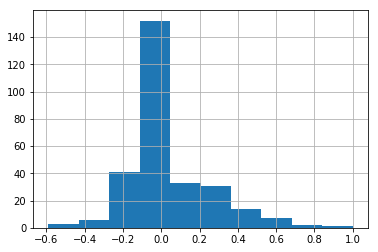
Max Correlation:  1.0
Min Correlation:  -0.589043523409763
Mean Correlation:  0.03910614218619199
Standard Deviation:  0.2129964043689813

SalePrice                1.000000
OverallQual              0.790982
GrLivArea                0.708624
GarageCars               0.640409
GarageArea               0.623431
TotalBsmtSF              0.613581
1stFlrSF                 0.605852
FullBath                 0.560664
BsmtQual_Ex              0.553105
TotRmsAbvGrd             0.533723
YearBuilt                0.522897
YearRemodAdd             0.507101
KitchenQual_Ex           0.504094
Foundation_PConc         0.497734
GarageYrBlt              0.486362
MasVnrArea               0.477493
Fireplaces               0.466929
ExterQual_Gd             0.452466
ExterQual_Ex             0.451164
BsmtFinType1_GLQ         0.434597
HeatingQC_Ex             0.434543
GarageFinish_Fin         0.419678
Neighborhood_NridgHt     0.402149
BsmtFinSF1               0.386420
SaleType_New             0.357509
SaleCondition_Partial    0.352060
LotFrontage              0.351799
FireplaceQu_Gd           0.339329
GarageType_Attchd        0.335961
MasVnrType_Stone         0.330476
                           ...
Fence_MnPrv             -0.140613
Neighborhood_BrkSide    -0.143648
SaleCondition_Normal    -0.153990
KitchenQual_Fa          -0.157199
Exterior1st_Wd Sdng     -0.158619
Exterior2nd_Wd Sdng     -0.161800
Exterior2nd_MetalSd     -0.162389
HouseStyle_1.5Fin       -0.163466
Neighborhood_IDOTRR     -0.164056
Exterior1st_MetalSd     -0.167068
Neighborhood_Edwards    -0.179949
Neighborhood_NAmes      -0.188513
Neighborhood_OldTown    -0.192189
Electrical_FuseA        -0.193978
Foundation_BrkTil       -0.204117
PavedDrive_N            -0.212630
RoofStyle_Gable         -0.224744
SaleType_WD             -0.242598
CentralAir_N            -0.251328
BsmtExposure_No         -0.263600
LotShape_Reg            -0.267672
MSZoning_RM             -0.288065
HeatingQC_TA            -0.312677
Foundation_CBlock       -0.343263
GarageType_Detchd       -0.354141
MasVnrType_None         -0.374468
GarageFinish_Unf        -0.410608
BsmtQual_TA             -0.452394
KitchenQual_TA          -0.519298
ExterQual_TA            -0.589044
Name: SalePrice, Length: 290, dtype: float64
So the if the correlation between the sale price and a feature is very small or close to zero, it's valid to say that such a feature has little to no influence on our price. The important features are going to be ones that have a significantly large enough absolute value of their correlation coefficient.
Thus we could specify a threshold of correlation that selects only features whose correlation with the SalePrice has an absolute value greater than that threshold. This could take a little bit of guess work, but we will try with a correlation greater than \(\|\pm0.4\|\).
Using the series of correlation coefficients just made, select all the ones with an absolute value greater than 0.4, and select the features corresponding to the coefficients. You should have 26 features. Call these features the key_features.
26
Now lets scatter plot each key feature compared to the sale price. This will allow us to detect things like skews in the data, which we can impute/transform in the following steps.
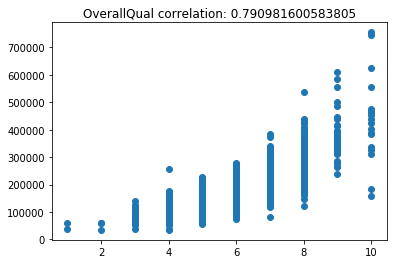
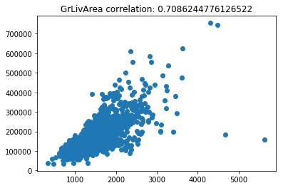
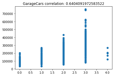
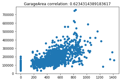
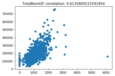
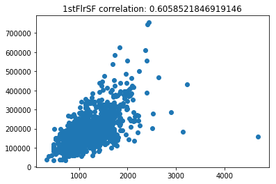
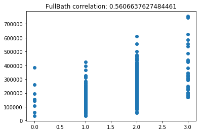
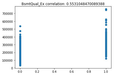
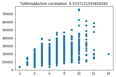
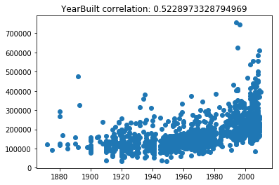
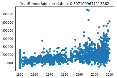
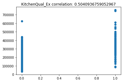
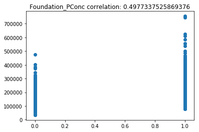
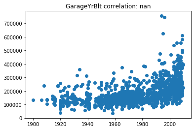
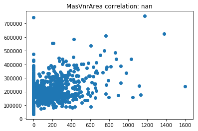
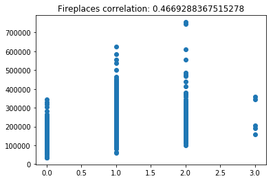
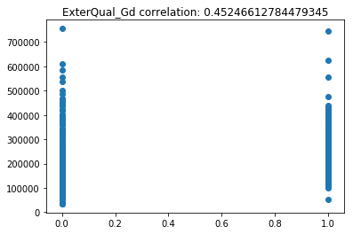
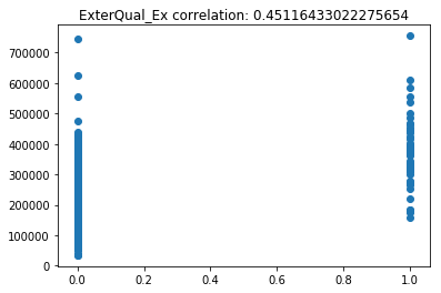
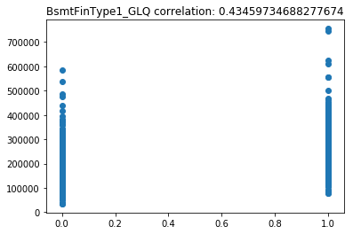
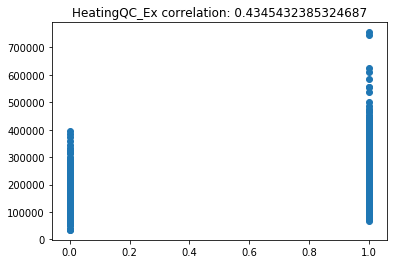
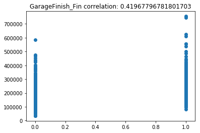
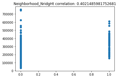
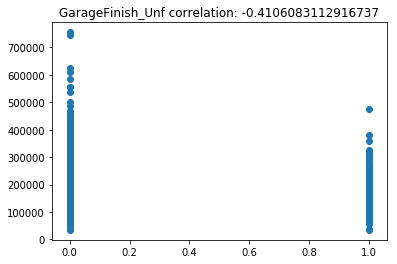
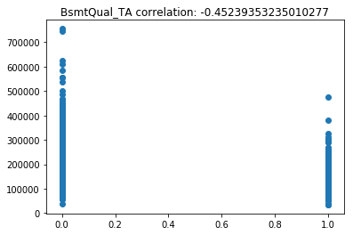
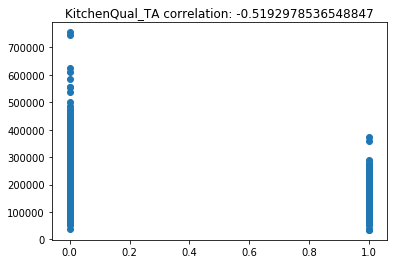
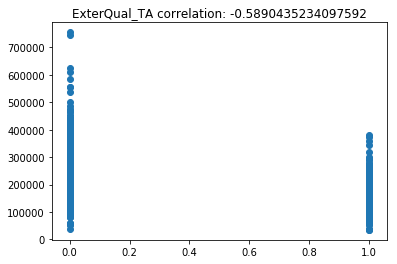
Its very obvious that some of these features are very skewed. Moreover, the magnitude of some of the features are on significantly different scales. For example, the values for GarageFinish_Unf have a range of 0 and 1, but the feature GarageYrBuilt ranges from 1900 to 2010. Machine learning models work best with unskewed data which is all on a similar scale.
So what can we do? We can use a data-transformation technique that allows us to get all the data on the same scale, and (hopefully) removes the skew in the data.
Do this in several steps:
- For the missing values in the original data frame, impute the mean value into each column.
- From
sklearn.preprocessing, useStandardScalerto transform our our columns into a standardized format
And what about our target variable, the SalePrice? Should it be transformed as well?
Using the seaborn function .distplot(data,fit=norm), plot the sale price. Below it, plot the stats.probplot(data,plot=plt) as well and see what it looks like. Make you have imported all the right things.
This accomplishes two tasks:
- Distplot will allow us to see how close our SalePrices are to a normal distribution, by creating a historgram.
- Probplot will allow us to see a Q-Q plot of our SalesPrices, generating a probability of sample data against the quantiles of a normal distribution.
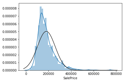
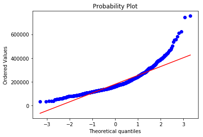
Now do the same thing again, but transform the SalePrice data with the function np.log1p(data).
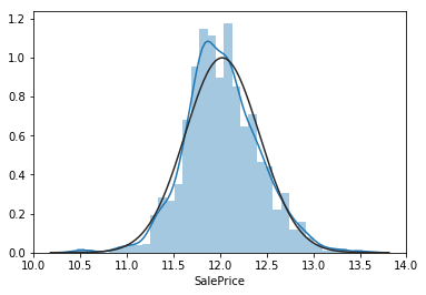
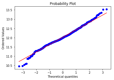
As we can see the transformation of np.log1p(y) makes our SalePrice data much more normal and minimizes skew. This is better for linear regression.
So what does this mean? It means that every price will be transformed such that \(y \rightarrow \ln(y+1)\)
This also means that when our model predicts values, we must transform it back to its original form to get the predicted price, using the inverse function \(\ln(y+1) \rightarrow e^{y}-1\), or
np.exp(y)-1.
V.Model Building
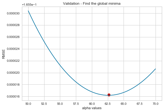
Ridge regression is one of the most common regularization techniques used in regession tasks. It is easy to use, and we'll let it be our model we work with. We need to fit it to our data to tune it's hyperparameter. We can find the right hyperparameter using cross validation.
- In the following cell, import Ridge and cross_val_score
- Create a function that returns the square root of a five fold cross validation of the negative value for the scoring metric.
scoring="neg_mean_squared_error" - Using the
np.linspace()function, create a series of values, between 50 and 70, that we will test as our hyperparameter alpha. - Create another series that finds that average cross validation score for each alpha.
- Make a matplotlib plot that has the alphas on the x-axis, and the RMSE on the vertical.
- For this to work, you should have used
StandardScaler()to transform the features, andnp.log1p(y)on theSalePrice. - Find the minimum value of alpha - this will be our hyperparameter.
If you did everything right, it should the plots should look like the next one:
Best alpha for ridge is: 62.6530612244898
VI.Model Development & Testing
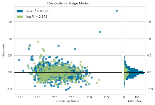
So now that we've cleaned data, selected the features, transformed them and found the right hyperparameter for our model, it's time to use test our model. Heres what we do next:
- Do a
train_test_splitwith a 77-33% split to test - Convert the predicted values into actual prices via the inverse function,
np.exp(y_pred)+1, and convert the test values of y to actual prices. - Plot the predicted prices vs the actual prices
- Plot the residuals of the predictions using the
ResidualsPlotfrom theyellowbricks.regressorpackage (install it if you dont have it)! - Using the yellow bricks plot, observe the normality of errors and R2 score of the train and test set!
If you did it correctly, your plot should looks like this:
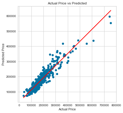
Your plot should look like this:
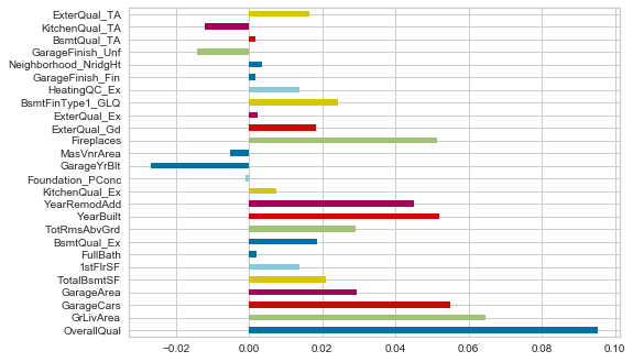
Lastly, make a horizontal bar plot of the coefficients in the ridge model.
* Use the attribute model.coef_ to get the coefficients. Put them into a series
Your plot should look like this.
VII.Sources & Credits
Some of these tutorials were very helpful in writing this lesson.
- https://www.kaggle.com/c/house-prices-advanced-regression-techniques#tutorials
- https://www.kaggle.com/pmarcelino/comprehensive-data-exploration-with-python
- https://www.kaggle.com/dgawlik/house-prices-eda
- https://www.kaggle.com/juliencs/a-study-on-regression-applied-to-the-ames-dataset
- https://www.kaggle.com/apapiu/regularized-linear-models