Before the Bitcoin Bubble Burst: Predicting day to day prices with ARIMA & Neural Nets
Joe Ganser
Abstract
The objective of this blog post is to experiment with time series techniques as well as methods in signal/noise extraction to make a prediction on the prices of both bitcoin and ethereum in the last week of August 2017, using all the previous pricing data.
In this short term price forecast, I am predicting the next day's price based upon all the prices leading upto it. Then on the next day, I am repeating this process again, once next day's price is received. Model techniques like this could be used for high frequency trading, not long term investing. This is NOT about predicting long term trends.
Because I am only predicting the next day out, and I am extracting the signal from the noise and what the models ACTUALLY predict is the noise. The predicted noise is then plugged back into the signal function, and that turns into the measurable prediction. This concept is explained a little more below.
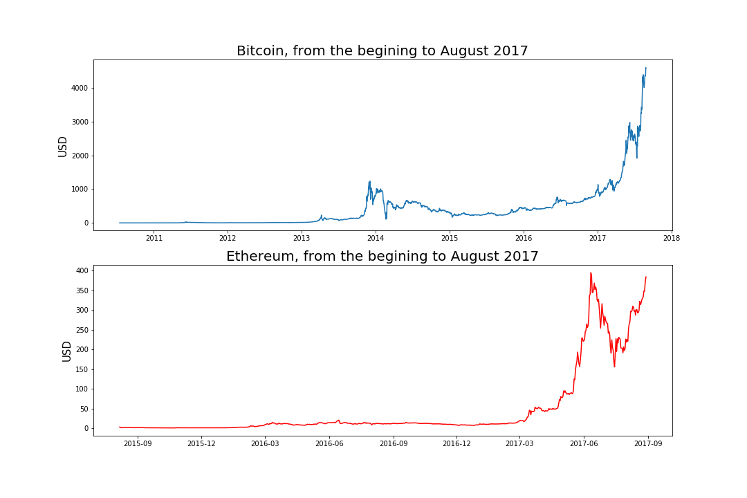
Lets take a look at the pricing data upto this point so far;
I.Introduction
WORKFLOW
The general process of how I built my models can be summarized in a few steps.
-
Extract the signal from the noise (find stationarity via dickey fuller test). More about this below.
-
Model the noise, and predict the noise for the next day (ARIMA and Neural nets)
-
Plug the predicted noise into the signal, calculating the price value for the next day
-
Compare the predicted price of the next day to the actual next day's price
-
Repeat steps 2 and 3 once when obtaining the actual price of the next day (use a for loop)
II.Model Choices: ARIMA & Neural Net Recursion
The model choice was done simply for comparitive experimental reasons, only because ARIMA and Neural Net LSTM can predict time series. Other techniques could be done to, but I just wanted to compare these out of curiosity. Their performance metrics were the cumulative root mean square error across all the days predicted.
ASSUMPTIONS
The assumption, which is validated, is that the exponential long term trend shall remain over the last few days of August of 2017. The assumption was made through the techniques of signal noise extraction which are explained below. I do NOT assume that the exponential trend will go on forever.
MODEL PREDICTIONS
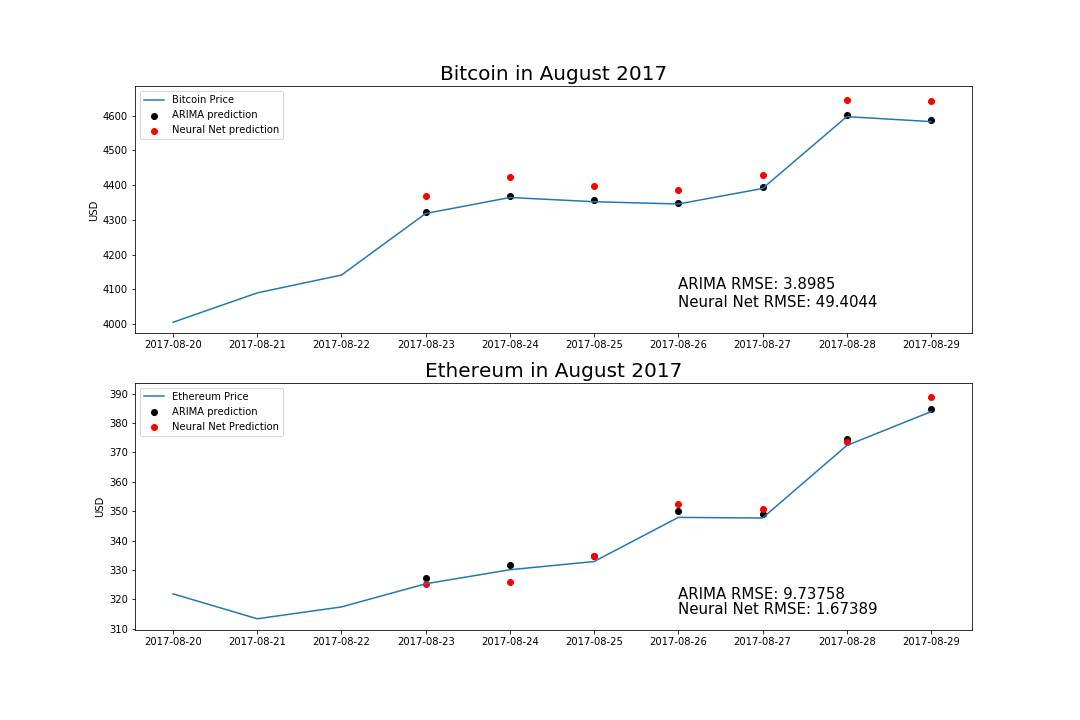
Here are the final results - the actual predictions of my models.
Predictions for Bitcoin
| Date | Bitcoin Price | ARIMA prediction | Neural Net Prediction |
|---|---|---|---|
| 2017-08-23 | 4318.35 | 4321.92 | 4369.75 |
| 2017-08-24 | 4364.41 | 4368.25 | 4423.16 |
| 2017-08-25 | 4352.30 | 4356.23 | 4397.79 |
| 2017-08-26 | 4345.75 | 4349.69 | 4384.69 |
| 2017-08-27 | 4390.31 | 4394.20 | 4430.15 |
| 2017-08-28 | 4597.31 | 4601.04 | 4643.98 |
| 2017-08-29 | 4583.02 | 4587.37 | 4643.36 |
Predictions for Ethereum
| Date | Ethereum Price | ARIMA prediction | Neural Net Prediction |
|---|---|---|---|
| 2017-08-23 | 325.28 | 327.39 | 325.36 |
| 2017-08-24 | 330.06 | 331.70 | 325.76 |
| 2017-08-25 | 332.86 | 334.69 | 334.74 |
| 2017-08-26 | 347.88 | 350.00 | 352.49 |
| 2017-08-27 | 347.66 | 348.96 | 350.64 |
| 2017-08-28 | 372.35 | 374.69 | 373.62 |
| 2017-08-29 | 383.86 | 384.72 | 388.87 |
III. Model Evluation
So looking at these results, what were the model performance metrics? The performance metric I used to compare the results of the techniques was the summed root mean square error across all the days (seven, in total) predicted.
| Model | Bitcoin RMSE | Ethereum RMSE |
|---|---|---|
| ARIMA | 3.8985 | 9.73758 |
| Neural Net | 49.40448 | 1.67389 |
Cumulative across the dates of Aug 23-Aug 29 2017.
Interesting Results!
ARIMA tended to perform better on bitcoin than neural nets, but the neural nets performed much better on the ethereum data! This may be related to the signal function I used, which is explained below.
EXTRACTING THE SIGNAL FROM THE NOISE USING THE AUGMENTED DICKEY FULLER TEST
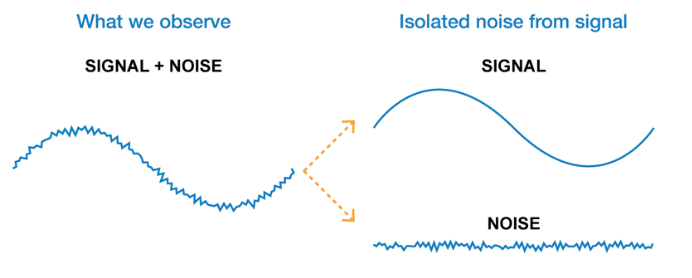
The augmented dickey fuller test is a statistical test to determine stationarity. Stationarity occurs when a series of data is transformed into format which clearly identifies the signal (aka a "trend") and all we are left with is noise. More specifically, stationarity occurs when we put the time series data is put into it's correct inverse function. With outputs similar to a Z-test, the test tells us if the new format we have has clearly identified the signal within the data. The null hypothesis of the Dickey Fuller test is that the signal and noise are NOT decoupled. The strategy behind using this is that by extracting the signal, we model and predict the noise and plug those predictions back into the signal.
Stationarity data has four fundamental criteria:

THE BEST FIT FUNCTION & IT'S INVERSE
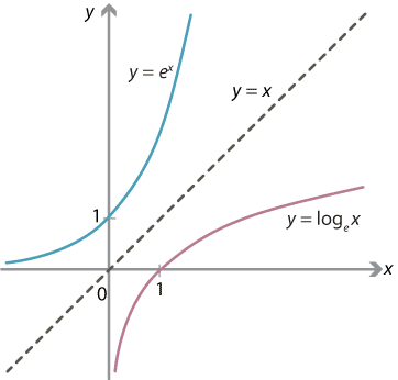
Knowing the best fitting function is not enough to model the time series. What is needed is not only a best fit function, but that function's inverse as well. By putting the data of the time series into the inverse function, we can get the noise values. It's noise values that are put into the Dickey Fuller test.
A graphical example of an inverse function: log(x) is the inverse of e^(x)
Extracting the signal from the noise can be summed into three steps
- Find the a function similar to the time series data.
- Find that function's inverse.
-
Plug the time series data into the inverse, and plug that transformed data set into the Dickey Fuller Test
*If we haven't rejected the null hypothesis in step 3 try step 1 over starting with a different function.
By looking at the very first plot, we can see that the trend of the cryptocurrency prices are in some way exponential. Thus, I can hypothesize that the signal is exponential in form.

The actual function form that allowed me to seperate the signal from the noise was indeed exponential in form but not simply exponential. It was by using this function's inverse that I could pass the dickey fuller test.
The actual function that worked was this:
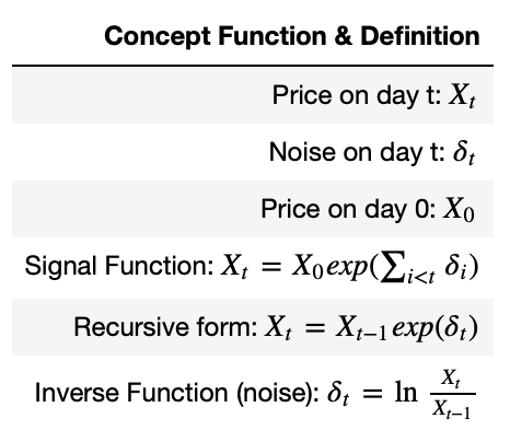
These function transformations worked with both the bitcoin & ethereum data.
In code form, it is:
noise = (np.log(data['Price'])-np.log(data['Price'].shift())).dropna()
Where the '.shift()' cooresponds to the day before.
FAILING AND THEN PASSING THE DICKEY FULLER TEST
In the images passing the Dickey Fuller test without perfmoring any transformation, and then (botton of each tab), the Dickey Fuller test is passed (meaning we can reject the null hypothesis, and the data is stationary.)
So now I have clearly identified the stationary form of the time series. These stationary forms can be plugged into the models to predict the noise, and using the noise predictions we can plug those back into the signal.
The plots below show the series, the rolling mean and standard deviations plotted side by side. The first is what the original series looked like, and the second is what the series looks like after it's input into the inverse transformation function.
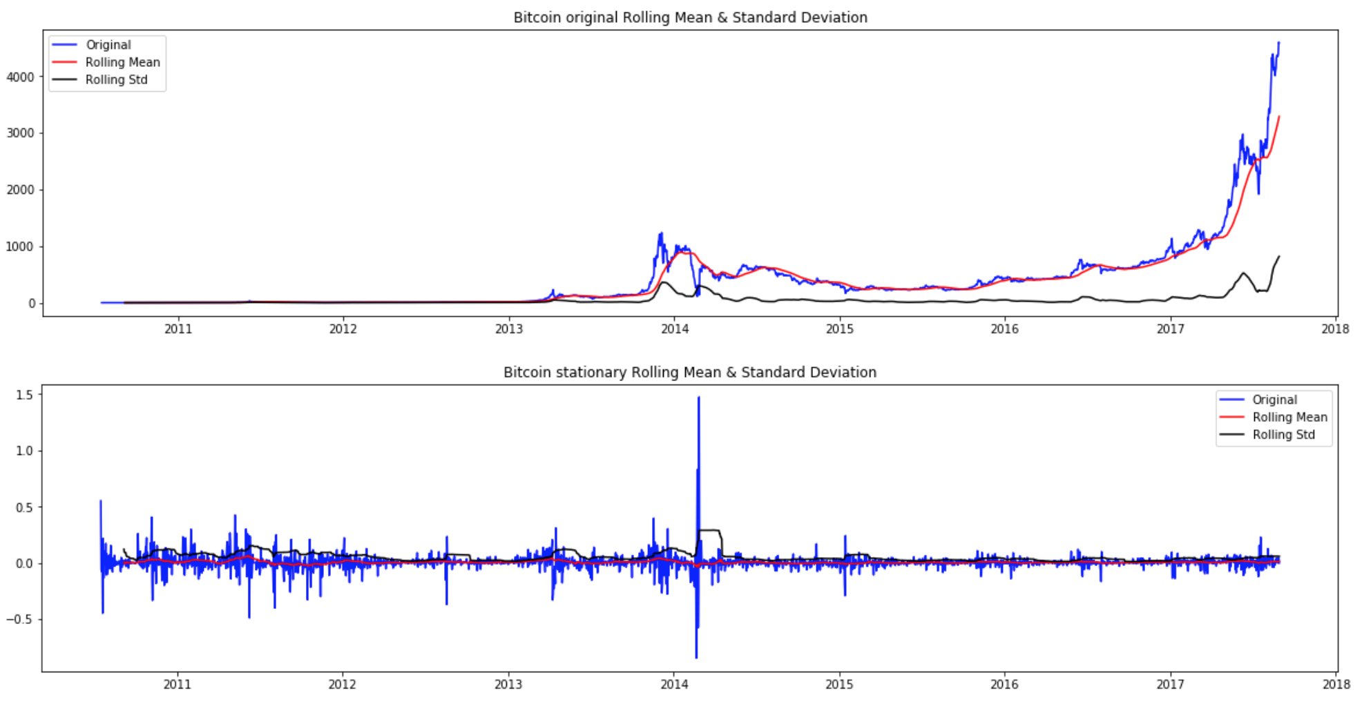
The specific statistics for the tests were:
Bitcoin Dickey-Fuller Test:|Results when transformed to stationary|Results results before stationary (failing) ------|---------|--------| Test Statistic|-20.254025|3.433511 p-value|0.000000|1.00000 Number Lags Used|4.000000|28.0000 Number of Observations Used| 2596.000000|2573.000000 Critical Value (1%)|-3.962262|-3.962293 Critical Value (5%)|-3.412183|-3.412198 Critical Value (10%)|-3.128047|-3.128055
IV: Model Code
So the prediction steps are structured in a FOR LOOP:
- Plug the noise into the model
- Train the model on the history of the noise
- Predict the noise of the next day
- Plug the next day's predicted noise into the signal function.
- Add the actual price of the next day to the price data set, transform it into stationarity and start again at step 1.
MODELLING WITH ARIMA
There are several steps to building an ARIMA model. ARIMA operates on three parameters. Based upon the plots of auto-correlation, partial auto-correlation and the amount of Bayesian information criterion we select these three parameters. Ofcourse, the end goal is to minimize the root mean squared error of the model.
AUTO CORRELATION & PARTIAL AUTOCORRELATION PLOTS
The plots of auto-correlation & partial auto-correlation for bitcoin & ethereums stationary formats were:

Using these plots I can estimate the ARIMA parameters (p,q) of the parameters (p,q,d) for ARIMA models. Just by looking at the graphs it can be estimate that p & q are around no more than 7 each. After grid searching through lots of combinations it was found that Bitcoins ARIMA parameters were (p=0,d=1,q=1) and Ethereum's ARIMA parameters were (p=2,d=0,q=0). These were validated by the minimization of the root mean squared error.
Here is the ARIMA model code:
def ARIMA_predictions(original_series,stationary_series,parameters, days_out):
    # Here we predict the noise
    train = stationary_series[:-days_out]
    # test the model on the last N points of the data, the models I used were at 7 days
    test = stationary_series[-days_out:]
    #
    history = [x for x in train]

    train.dropna(inplace=True)
    test.dropna(inplace=True)
    predicted_values = []
    tested = []

    #1. Plug the noise into the model
    #2. Train the model on the history of the noise
    #3. Predict the noise of the next day
    #4. Plug the next day's predicted noise into the signal function.
    #5. Add the actual price of the next day to the price data set, transform it into stationarity and start again at step 1.

    for i in range(len(test)):
        model = ARIMA(history, order=parameters)
        model_fit = model.fit(disp=0)
        yhat = float(model_fit.forecast(steps=1)[0])
        predicted_values.append(yhat)
        tested_values = list(test)[i]
        tested.append(tested_values)
        history.append(tested_values)
    predictions_series = pd.Series(predicted_values, index = test.index)

    # This part couples the signal to the noise.
    a = original_series.loc[original_series.index[-(days_out+1):]]['Price']
    b = np.exp(predictions_series)
    full_predictions = pd.DataFrame(a*b,columns=['Predicted with ARIMA']).dropna()
    df = pd.concat([original_series.loc[original_series.index[-days_out:]],full_predictions],axis=1)
    error = str(np.sqrt(mean_squared_error(df['Price'],df['Predicted with ARIMA'])))
    print("ARIMA Root Mean Squared Error: ",error)
    df.index.name = None
    df[['Price','Predicted with ARIMA']] = df[['Price','Predicted with ARIMA']].apply(lambda x: round(x,2))
    return df

bitcoin_ARIMA = ARIMA_predictions(bitcoin,bits_log_shift,(0,1,1),7)
Code for Neural Net LSTM
The neural net system was based upon sequential, dense LSTM modelling techniques. Like the ARIMA model, it was dependent upon a stationary time series input, modeling the noise and then putting the noise predictions back into the signal.
from sklearn.preprocessing import MinMaxScaler
from keras.models import Sequential
from keras.layers import Dense
from keras.layers import LSTM


def Neural_Net_predictions(original_time_series, stationary_time_series, days_out,nb_epoch,neurons):
    # note all these "sub" functions are used on the stationary time series.
    # The neural nets are used to predict the noise. Once the noise is predicted
    # Its plugged back into the signal

    X = stationary_time_series

    # Step 2
    # Break the time series into shifted components. Each column is a shifted value
    # previously in the time series
    def timeseries_to_supervised(data, lag=1):
        df = pd.DataFrame(data)
        columns = [df.shift(i) for i in range(1, lag+1)]
        columns.append(df)
        df = pd.concat(columns, axis=1)
        df.fillna(0, inplace=True)
        return df

    # Step 3
    # We must put the time series onto the scale acceptable by the activation functions
    def scale(train, test):
        scaler = MinMaxScaler(feature_range=(-1, 1))
        scaler = scaler.fit(train)
        train = train.reshape(train.shape[0],train.shape[1])
        train_scaled = scaler.transform(train)
        test = test.reshape(test.shape[0],test.shape[1])
        test_scaled = scaler.transform(test)
        return scaler, train_scaled, test_scaled


    # Step 4
    def fit_lstm(train, batch_size, nb_epoch, neurons):
        X, y = train[:, 0:-1], train[:, -1]
        X = X.reshape(X.shape[0], 1, X.shape[1])
        model = Sequential()
        model.add(LSTM(neurons, batch_input_shape=(batch_size, X.shape[1], X.shape[2]), stateful=True))
        model.add(Dense(1))
        model.compile(loss='mean_squared_error', optimizer='adam')
        for i in range(nb_epoch):
            model.fit(X, y, epochs=1, batch_size=batch_size, verbose=0, shuffle=False)
            model.reset_states()
        return model


    # Step 5
    def forecast_lstm(model, batch_size, X):
        X = X.reshape(1, 1, len(X))
        yhat = model.predict(X, batch_size=batch_size)
        return yhat[0,0]

    #Step 6
    def invert_scale(scaler, X, value):
        new_row = [x for x in X] + [value]
        array = np.array(new_row)
        array = array.reshape(1, len(array))
        inverted = scaler.inverse_transform(array)
        return inverted[0, -1]

    # Now use all the above functions
    supervised = timeseries_to_supervised(X,1)
    supervised_values = supervised.values
    train, test = supervised_values[0:-days_out], supervised_values[-days_out:]
    scaler, train_scaled, test_scaled = scale(train, test)
    train_reshaped = train_scaled[:,0].reshape(len(train_scaled),1,1)
    lstm_model = fit_lstm(train_scaled,1,nb_epoch,neurons)

    #Step 7
    predictions = []
    for i in range(len(test_scaled)):
        #Make one step forecast
        X, y = test_scaled[i,0:-1], test_scaled[i,-1]
        yhat = forecast_lstm(lstm_model,1,X)
        #invert scaling
        yhat = invert_scale(scaler, X, yhat)
        #store forecast
        predictions.append(yhat)

    # Step 8
    # This part plugs it back into the signal
    predictions_series = pd.Series(predictions, index = original_time_series.index[-days_out:])
    a = original_time_series.loc[original_time_series.index[-(days_out+1):]]['Price']
    b = np.exp(predictions_series)
    full_predictions = pd.DataFrame(a*b,columns=['Predicted with Neural Nets']).dropna()
    df = pd.concat([original_time_series.loc[original_time_series.index[-days_out:]],full_predictions],axis=1)
    error = str(np.sqrt(mean_squared_error(df['Price'],df['Predicted with Neural Nets'])))
    print("Neural Net Root Mean Squared Error: ",error)
    df.index.name=None
    df[['Price','Predicted with Neural Nets']] = df[['Price','Predicted with Neural Nets']].apply(lambda x: round(x,2))
    return df

bitcoin_NN = Neural_Net_predictions(bitcoin,bits_log_shift,days_out=7,nb_epoch=55,neurons=175)
V. Sources
-
The Application of Time Series Modelling and Monte Carlo Simulation: Forecasting Volatile Inventory Requirements By Robert Davies, Tim Coole, David Osipyw, https://file.scirp.org/pdf/AM_2014050513382674.pdf
-
How to Get Started with Deep Learning for Time Series Forecasting (7-Day Mini-Course), by Jason Brownlee; https://machinelearningmastery.com/how-to-get-started-with-deep-learning-for-time-series-forecasting-7-day-mini-course/
-
Statistical forecasting: notes on regression and time series analysis, By Robert Nau, Duke University https://people.duke.edu/~rnau/411arim.htm